Function Repository Resource:

BulirschEL2

Source Notebook

Evaluate Bulirsch's incomplete elliptic integral of the second kind

Contributed by: Jan Mangaldan

ResourceFunction["BulirschEL2"][x,m,a,b]

gives Bulirsch's incomplete elliptic integral of the second kind .

Details

Mathematical function, suitable for both symbolic and numerical manipulation.

Bulirsch’s incomplete elliptic integral of the second kind is defined as

When x=∞, ResourceFunction["BulirschEL2"] is referred to as a complete integral.

Argument conventions for elliptic integrals are discussed in "Elliptic Integrals and Elliptic Functions".

For certain special arguments, ResourceFunction["BulirschEL2"] automatically evaluates to exact values.

ResourceFunction["BulirschEL2"] can be evaluated to arbitrary precision.

ResourceFunction["BulirschEL2"] automatically threads over lists.

Examples

Basic Examples (1)

Evaluate numerically:

In[1]:=

Out[1]=

In[2]:=

$ResourceFunction["BulirschEL2"][\[Infinity], 0.7, 1.5, 1.8]$

Out[2]=

Scope (5)

Evaluate numerically for complex arguments:

In[3]:=

Out[3]=

Evaluate to high precision:

In[4]:=

Out[4]=

The precision of the output tracks the precision of the input:

In[5]:=

Out[5]=

Simple exact results are generated automatically:

In[6]:=

Out[6]=

In[7]:=

Out[7]=

BulirschEL2 threads elementwise over lists:

In[8]:=

Out[8]=

Series expansion of BulirschEL2 at the origin:

In[9]:=

Out[9]=

Applications (3)

Distance along a meridian of the Earth:

In[10]:=

$With[{a = UnitConvert[GeodesyData["ITRF00", "SemimajorAxis"]], e = GeodesyData["ITRF00", "Eccentricity"], \[Phi] = 23 \[Degree]}, a (1 - e^2) ResourceFunction["BulirschEL2"][Tan[\[Phi]], 1 - e^2, 1, 1 + e^2]]$

Out[10]=

Compare with the result of GeoDistance:

In[11]:=

Out[11]=

Calculate the surface area of a triaxial ellipsoid:

In[12]:=

$area[a_, b_, c_] := 2 \[Pi] (c^2 + (a^2 b)/Sqrt[a^2 - c^2] ResourceFunction["BulirschEL2"][Sqrt[a^2 - c^2]/c, ( c^2 (a^2 - b^2))/(b^2 (a^2 - c^2)), 1, c^2/b^2])$

The area of an ellipsoid with semiaxes 3, 2, 1:

In[13]:=

Out[13]=

Use RegionMeasure to calculate the surface area of the ellipsoid:

In[14]:=

Out[14]=

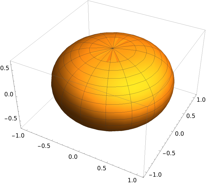
Parametrization of a Mylar balloon (two flat sheets of plastic sewn together at their circumference and then inflated):

In[15]:=

x[u_, v_] := Sqrt[(1 - u^2)/(1 + u^2)] Cos[v];
y[u_, v_] := Sqrt[(1 - u^2)/(1 + u^2)] Sin[v];
z[u_, v_] := ResourceFunction["BulirschEL2"][Sqrt[2] u/Sqrt[1 - u^2], 1/2, 1/
Sqrt[2], 0];

Plot the resulting balloon:

In[16]:=

$ParametricPlot3D[{x[u, v], y[u, v], z[u, v]}, {u, -1, 1}, {v, 0, 2 \[Pi]}, PlotRange -> All]$

Out[16]=

Properties and Relations (3)

Both incomplete and complete cases of EllipticE can be expressed in terms of BulirschEL2:

In[17]:=

$With[{\[Phi] = \[Pi]/5, m = 2/3}, N[{EllipticE[\[Phi], m], ResourceFunction["BulirschEL2"][Tan[\[Phi]], 1 - m, 1, 1 - m]}]]$

Out[17]=

In[18]:=

$With[{m = 2/3}, N[{EllipticE[m], ResourceFunction["BulirschEL2"][\[Infinity], 1 - m, 1, 1 - m]}]]$

Out[18]=

EllipticK and EllipticF can be expressed in terms of BulirschEL2:

In[19]:=

$With[{\[Phi] = \[Pi]/5, m = 2/3}, N[{EllipticF[\[Phi], m], ResourceFunction["BulirschEL2"][Tan[\[Phi]], 1 - m, 1, 1]}]]$

Out[19]=

In[20]:=

$With[{m = 2/3}, N[{EllipticK[m], ResourceFunction["BulirschEL2"][\[Infinity], 1 - m, 1, 1]}]]$

Out[20]=

BulirschEL2 can be used to represent linear combinations of elliptic integrals of the first and second kinds:

In[21]:=

$With[{a = 4, b = 5, \[Phi] = \[Pi]/5, m = 2/3}, N[{a EllipticF[\[Phi], m] + b EllipticE[\[Phi], m], ResourceFunction["BulirschEL2"][Tan[\[Phi]], 1 - m, a + b, a + b (1 - m)]}]]$

Out[21]=

In[22]:=

$With[{a = 4, b = 5, m = 2/3}, N[{a EllipticK[m] + b EllipticE[m], ResourceFunction["BulirschEL2"][\[Infinity], 1 - m, a + b, a + b (1 - m)]}]]$

Out[22]=

Neat Examples (1)

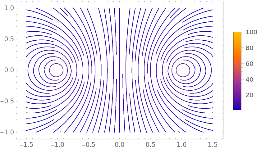
Magnetic field lines of a ring current in cylindrical coordinates:

In[23]:=

$With[{R = 1}, StreamPlot[{(2 z)/(r R ((r - R)^2 + z^2) Sqrt[(r + R)^2 + z^2]) ResourceFunction["BulirschEL2"][\[Infinity], 1 - (4 r R)/((r + R)^2 + z^2), 2 r R, 2 r R ((4 r R)/((r + R)^2 + z^2) - 1)], 2/(R ((r - R)^2 + z^2) Sqrt[(r + R)^2 + z^2]) ResourceFunction["BulirschEL2"][\[Infinity], 1 - (4 r R)/((r + R)^2 + z^2), 2 R (R - r), 2 R (r + R) (1 - (4 r R)/((r + R)^2 + z^2))]}, {r, -(3/2), 3/ 2}, {z, -1, 1}, {AspectRatio -> Automatic, PlotLegends -> Placed[Automatic, Right], StreamPoints -> Fine, StreamScale -> None}]]$

Out[23]=

Requirements

Wolfram Language 12.3 (May 2021) or above

Version History

1.0.0 – 22 June 2021

Source Metadata

Citation:
- Bulirsch R., "Numerical calculation of elliptic integrals and elliptic functions." Numerische Mathematik, vol. 7, no. 1, 78-90, 1965. DOI: 10.1007/BF01397975
- Bulirsch R., "Numerical calculation of elliptic integrals and elliptic functions. III." Numerische Mathematik, vol. 13, no. 4, 305-315, 1969. DOI: 10.1007/BF02165405

Related Resources

Author Notes

Requires 12.3 or later.

The form of the second argument was changed from the original definition used by Bulirsch, so that BulirschEL2 uses the parameter m=k² instead of the modulus k. This conforms with Mathematica's choice to use the parameter in the built-in elliptic integrals and functions.

License Information

This work is licensed under a Creative Commons Attribution 4.0 International License

Wolfram Function Repository

BulirschEL2

Details