Wolfram Function Repository
Instant-use add-on functions for the Wolfram Language
Function Repository Resource:
Generate a Krawtchouk matrix
ResourceFunction["KrawtchoukMatrix"][n] returns an n×n Krawtchouk matrix. |
A 4×4 Krawtchouk matrix:
| In[1]:= |
| Out[1]= |
Visualize the entries of a Krawtchouk matrix:
| In[2]:= |
| Out[2]= | 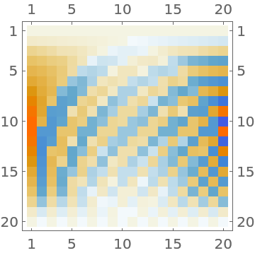 |
A normalized Krawtchouk matrix:
| In[3]:= |
| Out[3]= |  |
The normalized matrix is both symmetric and orthogonal:
| In[4]:= |
| Out[4]= |
By default, an exact matrix is computed:
| In[5]:= |
| Out[5]= |  |
Use machine precision:
| In[6]:= |
| Out[6]= |  |
Use arbitrary precision:
| In[7]:= |
| Out[7]= |  |
Define a symmetrized version of the Krawtchouk matrix:
| In[8]:= |
The symmetrized Krawtchouk matrix is symmetric, as its name implies:
| In[9]:= |
| Out[9]= |  |
| In[10]:= |
| Out[10]= |
The symmetrized Krawtchouk matrix gives the coefficients of the bivariate polynomial (1+x+y-x y)n-1:
| In[11]:= |
| Out[11]= |
Demonstrate a recursive method for generating the symmetrized Krawtchouk matrix:
| In[12]:= | ![With[{n = 7}, BlockMap[Total[#, 2] &, ArrayPad[
KroneckerProduct[symmetrizedKrawtchouk[n], {{1, 1}, {1, -1}}], 1], {2, 2}] == symmetrizedKrawtchouk[n + 1]]](https://www.wolframcloud.com/obj/resourcesystem/images/5c1/5c177871-288f-42a2-8aab-0ff17dbd8ac9/15b7d0cf66ffa03f.png) |
| Out[12]= |
The Kac matrix is a tridiagonal matrix whose subdiagonal and superdiagonal entries are consecutive integers:
| In[13]:= |
| In[14]:= |
| Out[14]= |  |
The Kac matrix can be diagonalized by the symmetrized Krawtchouk matrix:
| In[15]:= |
| Out[15]= |  |
Columns of the Krawtchouk matrix can be determined from the coefficients of the polynomial (1+x)n-j-1(1-x)j:
| In[16]:= |
| Out[16]= |
| In[17]:= |
| Out[17]= |
The entries of the Krawtchouk matrix can be expressed in terms of the Krawtchouk polynomial, which can be expressed in terms of Hypergeometric2F1:
| In[18]:= |
| Out[18]= |
| In[19]:= |
| Out[19]= |
Generate the Krawtchouk matrix through a recursive definition:
| In[20]:= | ![With[{n = 5}, Array[Which[#1 == 0, 1, #2 == 0, Binomial[n - 1, #1], True, #0[#1, #2 - 1] - #0[#1 - 1, #2] - #0[#1 - 1, #2 - 1]] &, {n,
n}, {0, 0}]]](https://www.wolframcloud.com/obj/resourcesystem/images/5c1/5c177871-288f-42a2-8aab-0ff17dbd8ac9/7da32514b469c481.png) |
| Out[20]= |
| In[21]:= |
| Out[21]= |
The product of a Krawtchouk matrix with itself is a constant multiple of the identity matrix of the same size:
| In[22]:= |
| Out[22]= |
Generate a Krawtchouk matrix from a Hadamard matrix, using condensation of the rows and columns with the same binary weights (number of 1's in the binary representation):
| In[23]:= | ![n = 7;
hm = 2^((n - 1)/2)
HadamardMatrix[2^(n - 1), Method -> "BitComplement"];
idx = Values[
KeySort[GroupBy[
Table[{k, DigitCount[k, 2, 1]}, {k, 0, 2^(n - 1) - 1}], Last -> First]]] + 1;
km = Table[Total[hm[[ji, ki]], 2], {ji, idx}, {ki, idx}] . DiagonalMatrix[1/Binomial[n - 1, Range[0, n - 1]]]](https://www.wolframcloud.com/obj/resourcesystem/images/5c1/5c177871-288f-42a2-8aab-0ff17dbd8ac9/5d192730feecb37b.png) |
| Out[24]= |
Verify that the result is a Krawtchouk matrix:
| In[25]:= |
| Out[25]= |
This work is licensed under a Creative Commons Attribution 4.0 International License