Function Repository Resource:

AntColonyOptimization

Source Notebook

Solve a combinatorial optimization problem using an Ant Colony Optimization (ACO) algorithm

Contributed by: Lars Ulke-Winter

ResourceFunction["AntColonyOptimization"][array,fitness]

returns the minimum found result for the function fitness with possible values for each variable given in array.

ResourceFunction["AntColonyOptimization"][array,fitness,All]

returns the intermediate optimization step results and optimization parameters as a summary Association.

Details and Options

ResourceFunction["AntColonyOptimization"] is a global stochastic optimization method for the solution of combinatorial arrangement problems. It imitates the swarm communication behaviour of ants during foraging (Stigmergic Optimization).

The optimization is based on the exchange of information between individuals (randomly generated solutions) using a virtual pheromone trail for the information exchange.

ResourceFunction["AntColonyOptimization"] finds a solution of vector x, where the i^th element of x is chosen from the values of the i^th list in array, such that fitness[x] has the smallest positive value found.

The input array takes a List of lists with available values at each row. The lists need not have uniform length.

The fitness function to be minimized must return a positive scalar value. Therefore, the standard method of negating the objective function to convert a minimization problem into a maximization problem doesn’t work in this ACO implementation.

Limitation: This implementation does not consider dependencies of design variables among each other. The assignment of the design variables must be independent of the settings of the others. The definition of the search space is therefore possible using only a given array and does therefore not require a given tree or graph structure of the search space. Optimization problems such as the traveling salesman cannot be encoded in this way.

Optimization parameters given as options include:

"PopulationSize"

500

number of ants

"MaxIterations"

200

maximum iterations

"FinishAtPheromoneThreshold"

0.95

stop criterion

"PheromoneFunction"

(1/#)&

pheromone concentration to be deposited depending on fitness

"WeatheringFactor"

0.05

fraction of decreasing pheromone concentration (selection probability) per iteration

"ProbabilitySelectBestPath"

0.02

proportion of generated solution alternatives that currently prefer the best solution

The computation will stop if the selection probability for a variable state exceeds the value of "FinishAtPheromoneThreshold".

"PheromoneFunction" is a function whose result marks the selection probability for the next step. By default, larger fitness results receive lower marking values than smaller fitness results.

Optimization parameters control the runtime behavior and solution quality as a tradeoff between exploitation and exploration. These can be modified depending on the target function and the number of variables, e.g. by trial and error.

The option "ProbabilitySelectBestPath" takes values between zero and one. Smaller values use probabilistic selecting resulting in slower convergence but exploring more possibilities.

The current minimal selection probability for a variable state is monitored during the iterations. The smaller it is, the greater the ability to explore new solutions.

The output of ResourceFunction["AntColonyOptimization"] is a List representing the best found solution. Due to the stochastic search method, this optimum does not necessarily have to be global, thus better solutions may exist.

When the third argument is All, the output is an Association with keys:

"Best"

variable allocation which minimizes fitness

"Iterations"

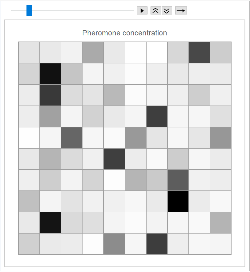
for each iteration step: {arguments which minimize fitness, normalized pheromone matrix, and current minimal selection probability for a variable state}

"NumberOfFunctionCalls"

number of calls made to the fitness calls

Examples

Basic Examples (2)

Create an array of possible assignments:

In[1]:=

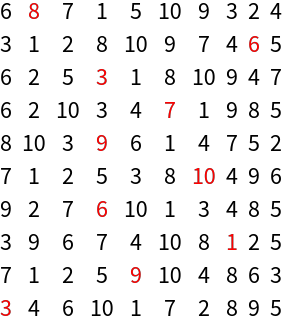
SeedRandom[314];
possibValues = Table[RandomSample[Range[10]], {i, Range[10]}];
possibValues // Grid

Out[3]=

Define an objective function to minimize:

In[4]:=

Search for minimum:

In[5]:=

Out[5]=

Return the complete iteration process using the third argument of All:

In[6]:=

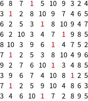
$SeedRandom[314]; possibValues = Table[RandomSample[Range[10]], {i, Range[10]}]; fit[x_List] := Total[x]$

In[7]:=

Out[5]=

Convergence behavior:

In[8]:=

Out[8]=

In[9]:=

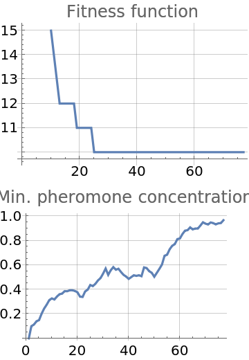
Column@{ListLinePlot[fit /@ result["Iterations"][[All, 1]], PlotLabel -> "Fitness function", GridLines -> Automatic],
ListLinePlot[result["Iterations"][[All, 3]], PlotLabel -> "Min. pheromone concentration", GridLines -> Automatic]}

Out[9]=

In[10]:=

Out[10]=

Options (4)

The above example with default options shown:

In[11]:=

In[12]:=

ResourceFunction["AntColonyOptimization"][
Table[RandomSample[Range[10]], {i, Range[10]}], Total[#] &, All,
"PopulationSize" -> 500, "MaxIterations" -> 200, "FinishAtPheromoneThreshold" -> 0.95, "WeatheringFactor" -> 0.05, "PheromoneFunction" -> (1/# &), "ProbabilitySelectBestPath" -> 0.02];

In[13]:=

Out[13]=

In[14]:=

Out[14]=

FinishAtPheromoneThreshold (1)

Terminate if a quarter of individuals have the same fitness value:

In[15]:=

In[16]:=

In[17]:=

Out[17]=

In[18]:=

Out[18]=

ProbabilitySelectBestPath (1)

Have 50% of the individuals select the current shortest path (low exploration):

In[19]:=

In[20]:=

In[21]:=

Out[21]=

In[22]:=

Out[22]=

PheromoneFunction (1)

Use a lower pheromone marking at each step depending on individual fitness value (low convergence speed, high exploration):

In[23]:=

In[24]:=

ResourceFunction["AntColonyOptimization"][
Table[RandomSample[Range[10]], {i, Range[10]}], Total[#] &, All,
"PheromoneFunction" -> (1/(20 #) &)];

In[25]:=

Out[25]=

In[26]:=

Out[26]=

WeatheringFactor (1)

Reduce the selection probability for less-used paths more slowly:

In[27]:=

In[28]:=

In[29]:=

Out[29]=

In[30]:=

Out[30]=

Applications (5)

How much money is in your pocket (knapsack problem)? (5)

Total given mass:

In[31]:=

Values for individual coins:

In[32]:=

In[33]:=

Fitness function (error function). In this problem the difference between the target coin weight and the calculated coin weight is minimized:

In[34]:=

$massError[coins_List] := Module[{eps = 10.^-6, error}, error = QuantityMagnitude[Abs@((Values[moneyMass] . coins) - mWallet), "Grams"]; If[(Total@coins) == 0, 10000., If[error <= eps, eps, error]]]$

Matrix of possible coins in wallet:

In[35]:=

possibCoins = Values@<|"1¢Range" -> Range[0, 5], "2¢Range" -> Range[0, 5], "5¢Range" -> Range[0, 5], "10¢Range" -> Range[0, 8], "20¢Range" -> Range[0, 7], "50¢Range" -> Range[0, 7], "1€Range" -> Range[0, 7], "2€Range" -> Range[0, 7]|>;
possibCoins // Grid

Out[8]=

Three optimization runs:

In[36]:=

Table[Values[
moneyMass] . (result = (ResourceFunction["AntColonyOptimization"][
possibCoins, massError, "PopulationSize" -> 1000, "FinishAtPheromoneThreshold" -> 0.99, "WeatheringFactor" -> 0.01, "MaxIterations" -> 30])) -> Values[moneyValue] . result,
{3}]

Out[36]=

Properties and Relations (1)

The fitness function must return a positive value. For maximization problems, fitness must be adjusted:

In[37]:=

ResourceFunction["AntColonyOptimization"][
{
{4, 2, 3, 1, 5, 6},
{3, 1, 6, 4},
{6, 3, 4, 1, 2, 5},
{6},
{5, 6},
{2, 6, 1}
},
(Total[1/#] &)]

Out[37]=

Neat Examples (7)

Minimize the mass of a rod structure (7)

Optimize a structure geometry:

In[38]:=

In[39]:=

In[40]:=

In[41]:=

Out[41]=

In[42]:=

Restrictions:

In[43]:=

In[44]:=

In[45]:=

Out[45]=

Define helper functions:

In[46]:=

$addSubMatrix[orgM_?MatrixQ, subM_?MatrixQ, atX_Integer, atY_Integer] := Module[{M = orgM, M1 = subM, rows = Length[subM], columns = Length[ Part[subM, 1]], i, j}, For[i = 1, i <= rows, For[j = 1, j <= columns, Part[M, atX - 1 + i, atY - 1 + j] = Part[ M, atX - 1 + i, atY - 1 + j] + Part[M1, i, j]; Increment[ j]]; Increment[i]]; M]$

In[47]:=

$generateStiffnesMatrix[ section_List] := Module[{stiff, rodelements, rodProp, rodLength, kSub, allStiff, c, s}, stiff = 10000.; rodelements = {{1, {1, 2, stiff, Part[section, 1]}}, {2, {1, 3, stiff, Part[section, 2]}}, {3, {2, 4, stiff, Part[section, 3]}}, {4, {4, 3, stiff, Part[section, 4]}}, {5, {1, 4, stiff, Part[section, 5]}}, {6, {2, 3, stiff, Part[section, 6]}}, {7, {3, 5, stiff, Part[section, 7]}}, {8, {5, 6, stiff, Part[section, 8]}}, {9, {4, 6, stiff, Part[section, 9]}}, {10, {3, 6, stiff, Part[section, 10]}}, {11, {4, 5, stiff, Part[section, 11]}}, {12, {5, 7, stiff, Part[section, 12]}}, {13, {7, 8, stiff, Part[section, 13]}}, {14, {6, 8, stiff, Part[section, 14]}}, {15, {5, 8, stiff, Part[section, 15]}}, {16, {6, 7, stiff, Part[section, 16]}}, {17, {7, 9, stiff, Part[section, 17]}}, {18, {8, 9, stiff, Part[section, 18]}}}; rodProp = ReplaceAll[rodelements, { Pattern[no, Blank[Integer]], Pattern[prop, Blank[List]]} :> {no, {c = (Part[nodes, Part[prop, 2], 2, 1] - Part[nodes, Part[prop, 1], 2, 1])/(rodLength = Sqrt[(Part[nodes, Part[prop, 2], 2, 1] - Part[nodes, Part[prop, 1], 2, 1])^2 + (Part[nodes, Part[prop, 2], 2, 2] - Part[nodes, Part[prop, 1], 2, 2])^2]), s = (Part[nodes, Part[prop, 2], 2, 2] - Part[nodes, Part[prop, 1], 2, 2])/rodLength, Part[prop, 3] (Part[prop, 4]/rodLength)}}]; kSub = ReplaceAll[ rodProp, { Pattern[no, Blank[Integer]], Pattern[prop, Blank[List]]} :> {no, Part[prop, 3] ReplaceAll[{{c1^2, c1 s1}, {c1 s1, s1^2}}, {c1 -> Part[ prop, 1], s1 -> Part[prop, 2]}]}]; allStiff = Table[ Table[0, {i, 1, 2 Length[nodes]}], {j, 1, 2 Length[nodes]}]; For[ i = 1, i <= Length[rodelements], allStiff = addSubMatrix[allStiff, Part[kSub, i, 2], Part[rodelements, i, 2, 1] 2 - 1, Part[rodelements, i, 2, 1] 2 - 1]; allStiff = addSubMatrix[ allStiff, -Part[kSub, i, 2], Part[rodelements, i, 2, 1] 2 - 1, Part[rodelements, i, 2, 2] 2 - 1]; allStiff = addSubMatrix[ allStiff, -Part[kSub, i, 2], Part[rodelements, i, 2, 2] 2 - 1, Part[rodelements, i, 2, 1] 2 - 1]; allStiff = addSubMatrix[ allStiff, Part[kSub, i, 2], Part[rodelements, i, 2, 2] 2 - 1, Part[rodelements, i, 2, 2] 2 - 1]; Increment[i]]; allStiff]$

In[48]:=

$computeMass[ section_List] := Module[{length = {20, 20, 20, 20, 20 Sqrt[2], 20 Sqrt[2], 20, 10, 10 Sqrt[5], 10 Sqrt[5], 20 Sqrt[2], 20, 10, 20, 10 Sqrt[5], 10 Sqrt[5], 20, 10 Sqrt[5]}}, Dot[length, section]]$

In[49]:=

$computeDeformation[ section_List] := Module[{sol, allStiff, uAll, unKnown, allForces, freac1, freac3, freac4, u2, u5, u6, u7, u8, u9, u10, u11, u12, u13, u14, u15, u16, u17, u18}, allStiff = generateStiffnesMatrix[ section]; uAll = {0, u2, 0, 0, u5, u6, u7, u8, u9, u10, u11, u12, u13, u14, u15, u16, u17, u18}; unKnown = {freac1, freac3, freac4, u2, u5, u6, u7, u8, u9, u10, u11, u12, u13, u14, u15, u16, u17, u18}; allForces = {freac1, 0, freac3, freac4, 0, 0, 0, 0, 0, 0, 0, 0, 0, 0, 0, 0, 0, -force}; sol = Flatten[ Solve[Dot[allStiff, uAll] == allForces, unKnown]]]$

The fitness function uses a penalty term to enforce constraints:

In[50]:=

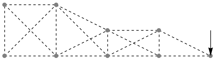
$objective[sections_] := With[{uMax = maxDeform, u18 = N@Abs@(computeDeformation[sections] // Last // Values), m = N@computeMass[sections]}, If[u18 > uMax, m + 250 (u18 - uMax)^2, m] ];$

Search for minimum mass structure according to the displacement constraints:

In[51]:=

result = ResourceFunction["AntColonyOptimization"][
ConstantArray[rodSectionsValid, Length@rodElements],
objective, "PopulationSize" -> 800, "MaxIterations" -> 20, "FinishAtPheromoneThreshold" -> 0.80];

Show the result:

In[52]:=

Out[52]=

In[53]:=

Out[53]=

In[54]:=

Out[54]=

Plot the result with deformed structure:

In[55]:=

solUAll = Partition[{0, Subscript[u, 2], 0, 0, Subscript[u, 5], Subscript[u, 6], Subscript[u, 7], Subscript[u, 8], Subscript[u, 9], Subscript[
u, 10], Subscript[u, 11], Subscript[u, 12], Subscript[u, 13], Subscript[u, 14], Subscript[u, 15], Subscript[u, 16], Subscript[
u, 17], Subscript[u, 18]} /. Thread[{Subscript[u, 2], Subscript[u, 5], Subscript[u, 6], Subscript[u, 7], Subscript[u, 8], Subscript[u, 9], Subscript[u,
10], Subscript[u, 11], Subscript[u, 12], Subscript[u, 13], Subscript[u, 14], Subscript[u, 15], Subscript[u, 16], Subscript[u, 17], Subscript[u, 18]} -> Values[computeDeformation[result]][[4 ;; -1]]], 2];

In[56]:=

In[57]:=

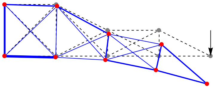
$structDeformed = Graphics[{rodElements /. {no_Integer, prop_List} :> {Blue, AbsoluteThickness[ prop[[3]] /. Table[Subscript[a, i] -> result[[i]]/10, {i, 18}]], Line[{defNodes[[prop[[1]], 2]], defNodes[[prop[[2]], 2]]}]}, defNodes /. {no_Integer, coord_List} -> {Hue[0], PointSize[0.02`], Point[coord]}}, AspectRatio -> Automatic];$

In[58]:=

Out[58]=

Publisher

Lars Ulke-Winter

Version History

1.0.0 – 13 February 2020

Source Metadata

Citation:
- Dorigo, M., "Optimization, Learning and Natural Algorithms." PhD thesis, Politecnico di Milano, Italy, 1992.

Related Resources

Author Notes

Detailed explanation what is being optimized in the first example:

The array (called possibValues in the Basic Examples section) shows the valid variable assignments in each row. Each row stands for one variable with its corresponding possible values. In this example you have 10 variables, each of which can have 10 different states. This results in 10¹⁰ possible variable assignments (the size of the search space in this example).

The optimization task is to find the shortest path (the minimum) through array (with its 10¹⁰ different permissible configurations) with regard to the defined function fit. For the sake of simplicity, the total value of the individual variables was simply chosen as the objective function in this example, fit=Total[#]&. Thus, for example, a path as marked in red here has a corresponding path length of Total[{3,9,1,6,10,9,7,3,6,8}]→62:

The optimal (shortest possible) path to be found by the AntColonyOptimization algorithm after some iterations is the following, which achieves Total[{1,1,1,1,1,1,1,1,1,1}]→10 as the absolute minimum of the search space:

This example is rather trivial and only serves to outline the basic procedure and introduce the basic parameters, (such as array and fitness) that are necessary to formulate the optimization problem. Slightly more complex application examples are demonstrated in the various Example subsections above.

A brief summary:

array (a list of lists) defines the search space, where the number of rows corresponds to the number of variables and the number of columns corresponds to the possible individual states of each variable. The number of possible variable states can generally be different for each variable.

The function fitness assigns each valid variable configuration an associated quantity, the corresponding path length. This allows comparison of the different variable configurations.

Within the given search space (encoded in array) and the given virtual path length (defined by fitness), AntColonyOptimization tries to find the shortest path (the minimum) through the search space. It returns the related variable assignments.

License Information

This work is licensed under a Creative Commons Attribution 4.0 International License

Wolfram Function Repository

AntColonyOptimization

Details and Options

Examples

Basic Examples (2)

Options (4)

FinishAtPheromoneThreshold (1)

ProbabilitySelectBestPath (1)

PheromoneFunction (1)

WeatheringFactor (1)

Applications (5)

How much money is in your pocket (knapsack problem)? (5)

Properties and Relations (1)

Neat Examples (7)

Minimize the mass of a rod structure (7)

Publisher

Related Links

Version History

Source Metadata

Related Resources

Author Notes

Detailed explanation what is being optimized in the first example:

A brief summary:

License Information

AntColonyOptimization

Details and Options

Examples

Basic Examples (2)

Options (4)

FinishAtPheromoneThreshold (1)

ProbabilitySelectBestPath (1)

PheromoneFunction (1)

WeatheringFactor (1)

Applications (5)

How much money is in your pocket (knapsack problem)? (5)

Properties and Relations (1)

Neat Examples (7)

Minimize the mass of a rod structure (7)

Publisher

Related Links

Version History

Source Metadata

Related Resources

Related Symbols

Author Notes

Detailed explanation what is being optimized in the first example:

A brief summary:

License Information