Details
ResourceFunction["BlockEntropy"] is similar to
Entropy in that it also computes values from a sum of the form
-∑piLog[pi].
The entropy measurement starts with grouping rows by
Total.
Typically, pi is a frequentist probability of obtaining the ith distinct element by randomly sampling the input list.
ResourceFunction["BlockEntropy"] expects a matrix structure, either of the form data={row1,row2,…}, or implicitly as Partition[list,blocksize] ={row1,row2,…}.
Additionally, BlockEntropy allows for coarse-graining of rows to macrostates using the function
macrofun (default:
Total).
Two rows rowj and rowk, with macrostates mj=macrofun[rowj] and mk=macrofun[rowk], are considered distinct if mj≠mk.
Likewise, two atomistic states dj,x and dk,y are considered distinct if dj,x≠dk,y.
Let 𝒟 be the set of unique atomistic states and ℳ the set of distinct values in the range of macrofun. The joint entropy is then calculated by a double sum, S=-∑ℙ(dj❘mi)ℙ(mi)Log[ℙ(dj❘mi)ℙ(mi)], where indices i and j range over the elements of ℳ and 𝒟 respectively.
The frequentist probability ℙ(mi) , mi∈ℳ equals the count of rows satisfying mi=macrofun[rowj], divided by the total number of rows.
The conditional probability ℙ(dj❘mi), mi∈ℳ, dj∈𝒟 is not necessarily frequentist, but is often assumed or constructed to be so.
The optional function
probfun takes
mi∈ℳ as the first argument and
blocksize as the second argument. It should return an
Association or
List of conditional probabilities
ℙ(dj❘mi).
When probfun is not set, either "Micro" or "Macro" conditional probabilities can be specified by setting the "Statistics" option.
The default "Micro" statistics obtains 𝒟 by taking a
Union over row elements. The conditional probabilities are then calculated as
ℙ(dj❘mi)=∑ℙ(dj❘rowk)ℙ(rowk)=∑ℙ(dj❘rowk) /N, where the sum includes every possible
rowk written over elements 𝒟 and satisfying
mi=macrofun[rowk]. The factor
1/ℙ(rowk)=N equals the
Count of such rows, all assumed equiprobable.
Traditional "Macro" statistics require that 𝒟 contains all possible rows of the correct length whose elements are drawn from the complete set of row elements using
Tuples. The conditional probabilities are then calculated as
ℙ(dj❘mi)=0 if
mi≠macrofun[dj] or if
mi=macrofun[dj] as
ℙ(dj❘mi)=1 /N, with
N equal to the count of atomistic row states
dk satisfying
mi=macrofun[dk].
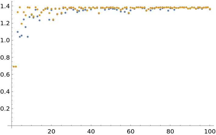
![ListPlot[Transpose[Abs[List[
ResourceFunction["BlockEntropy"][SeedRandom[Floor[10^6 Pi^#]];
RandomInteger[1, {#, 2}], Total],
ResourceFunction["BlockEntropy"][SeedRandom[Floor[10^6 Pi^#]];
RandomInteger[1, {#, 2}], Entropy]
]] & /@ Range[100]], PlotRange -> All]](https://www.wolframcloud.com/obj/resourcesystem/images/569/569937ec-536d-4980-820d-889f03a1a414/24fdc6122fbc774d.png)
![ResourceFunction["BlockEntropy"][CompoundExpression[
SeedRandom[144234], RandomInteger[5, 100]
], 5, Total, Function[{any}, {1}]]](https://www.wolframcloud.com/obj/resourcesystem/images/569/569937ec-536d-4980-820d-889f03a1a414/6494310c67885926.png)
![With[{rand = CompoundExpression[
SeedRandom[144234],
RandomInteger[5, 100]]},
Equal[ResourceFunction["BlockEntropy"][rand, 5, Total,
Function[{any}, {1}]],
Entropy[Total /@ Partition[rand, 5]]]]](https://www.wolframcloud.com/obj/resourcesystem/images/569/569937ec-536d-4980-820d-889f03a1a414/33e6f8385096e390.png)
![Map[# -> ResourceFunction["BlockEntropy"][SeedRandom[324313];
RandomInteger[2, 12], 3,
"Statistics" -> #] &,
{"Micro", "Macro"}] // Column](https://www.wolframcloud.com/obj/resourcesystem/images/569/569937ec-536d-4980-820d-889f03a1a414/7580ef7f3463415b.png)
![N[Subtract[ResourceFunction["BlockEntropy"][
RandomInteger[2, 10^6 + 2], 3,
"Statistics" -> "Macro"], Log[3^3]]]](https://www.wolframcloud.com/obj/resourcesystem/images/569/569937ec-536d-4980-820d-889f03a1a414/26fdb05b5b3e7bce.png)
![ListLinePlot[Outer[N@ResourceFunction["BlockEntropy"][
Table[PadLeft[{1}, #2], 10],
"Statistics" -> #1] &,
{"Micro", "Macro"}, Range[2, 10], 1]]](https://www.wolframcloud.com/obj/resourcesystem/images/569/569937ec-536d-4980-820d-889f03a1a414/360f998b5196e019.png)
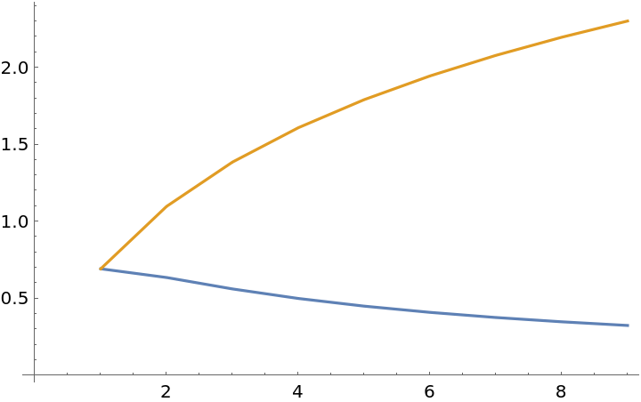
![ListLinePlot[Transpose[{
-1/# Log[1/#] - (# - 1)/# Log[(# - 1)/#],
-Log[1/#]} & /@ Range[2, 10]]]](https://www.wolframcloud.com/obj/resourcesystem/images/569/569937ec-536d-4980-820d-889f03a1a414/675bc44589491dc8.png)

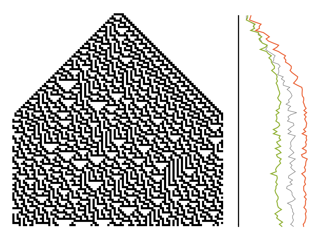
![ImageRotate[GraphicsColumn[{ListLinePlot[{
0 & /@ #,
Entropy[Partition[#, 5]] & /@ #,
ResourceFunction["BlockEntropy"][#, 5, "Statistics" -> "Micro"] & /@ #,
ResourceFunction["BlockEntropy"][#, 5, "Statistics" -> "Macro"] & /@ #
}, PlotStyle -> {
Directive[Thickness[0.005], Black],
Directive[Thickness[0.0025], Gray],
Automatic, Automatic},
Ticks -> False, Axes -> False,
ImageSize -> {400, Automatic},
AspectRatio -> 1/3], ArrayPlot[
Transpose[#], Frame -> None,
ImageSize -> {400, Automatic}]
} &@CellularAutomaton[30,
CenterArray[{1, 1, 1, 1, 1}, 100], 100]], -Pi/2]](https://www.wolframcloud.com/obj/resourcesystem/images/569/569937ec-536d-4980-820d-889f03a1a414/0684a00dfd6bf26f.png)
![With[{rand = RandomInteger[2, 25]},
Equal[Entropy[Partition[rand, 5]],
ResourceFunction["BlockEntropy"][rand, 5, Identity,
"Statistics" -> "Macro"]]]](https://www.wolframcloud.com/obj/resourcesystem/images/569/569937ec-536d-4980-820d-889f03a1a414/2189d886372d0fdb.png)
![SeedRandom[1234];
Equal[ResourceFunction["BlockEntropy"][RandomSample /@ Table[#, 5]],
Entropy[#]] &@RandomInteger[2, 5]](https://www.wolframcloud.com/obj/resourcesystem/images/569/569937ec-536d-4980-820d-889f03a1a414/4fd0f4a4efe64bb8.png)
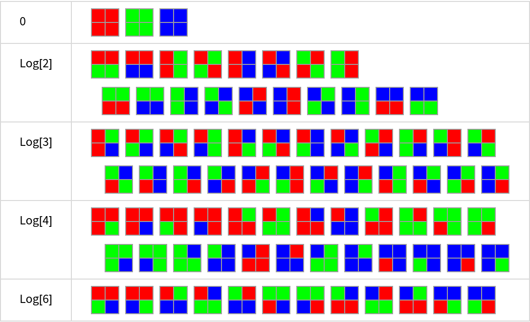
![Grid[KeyValueMap[{#1, Row[#2, Spacer[1]]} &,
Map[ArrayPlot[Partition[#, 2], Mesh -> True, ImageSize -> 30,
ColorRules -> {a -> Red, b -> Green, c -> Blue}] &,
KeySort[
GroupBy[Tuples[{a, b, c}, 4], ResourceFunction["BlockEntropy"][#, 2, Entropy] &],
NumericalOrder], {2}]], Frame -> All, FrameStyle -> LightGray,
Alignment -> Left, Spacings -> {3, 1}]](https://www.wolframcloud.com/obj/resourcesystem/images/569/569937ec-536d-4980-820d-889f03a1a414/05db849f5ab098aa.png)
![N[Subtract[
ResourceFunction["BlockEntropy"][
First[RealDigits[Pi, 2, #*100000]],
#, Total, "Statistics" -> "Macro"], Log[2^#]]] & /@ Range[2, 5]](https://www.wolframcloud.com/obj/resourcesystem/images/569/569937ec-536d-4980-820d-889f03a1a414/5111cf36a3d7c373.png)