Wolfram Function Repository
Instant-use add-on functions for the Wolfram Language
Function Repository Resource:
Compute the apparent visual shape of an object or region traveling with constant velocity
ResourceFunction["RelativisticInertialDeformedRegion"][region,speed,tObs,accuracyGoal] gives the deformed visual shape of region, intially positioned at the origin,traveling at speed along the positive x-axis, at time tObs and with an accuracy of accuracyGoal. | |
ResourceFunction["RelativisticInertialDeformedRegion"][region,speed,θ,ϕ,tObs,accuracyGoal] gives the deformed visual shape when region is traveling in the direction defined by spherical coordinates θ and ϕ. | |
ResourceFunction["RelativisticInertialDeformedRegion"][region,vec,speed,θ,ϕ,tObs,accuracyGoal] gives the deformed visual shape when region is intially positioned at vec. |
Compute the apparent shape of a sphere with radius 2 moving with speed 0.9 in the positive x direction, as observed at different times:
| In[1]:= | ![GraphicsRow[
Table[ResourceFunction["RelativisticInertialDeformedRegion"][
Sphere[], 0.9, time, 100], {time, -6, 6, 3}]]](https://www.wolframcloud.com/obj/resourcesystem/images/55e/55ed74f8-de0e-4441-9c14-f5b4fbcbc450/0d884b889c6e6732.png) |
| Out[1]= | 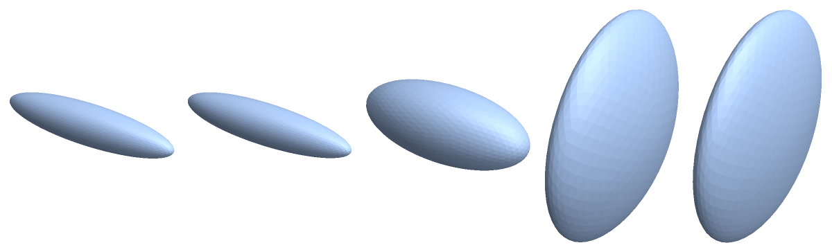 |
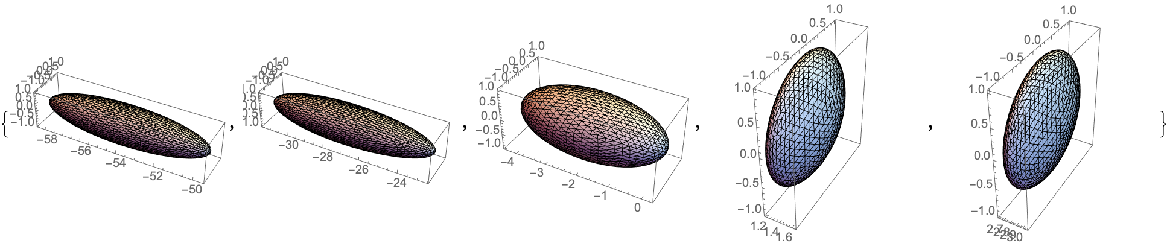
If we use Graphics3D with visible axes, we can see that the sphere is only stretched or contracted in the x direction:
| In[2]:= | ![Table[Graphics3D[
ResourceFunction["RelativisticInertialDeformedRegion"][Sphere[], 0.9, time, 100], Axes -> True], {time, -6, 6, 3}]](https://www.wolframcloud.com/obj/resourcesystem/images/55e/55ed74f8-de0e-4441-9c14-f5b4fbcbc450/4fe53685f8f01b31.png) |
Move the sphere diagonally up and to the right, with a speed of 0.7:
| In[3]:= | ![Graphics3D[
Table[ResourceFunction["RelativisticInertialDeformedRegion"][
Sphere[], 0.7, \[Pi]/2, \[Pi]/2 + \[Pi]/4, time, 100], {time, -6, 6, 3}], Axes -> True]](https://www.wolframcloud.com/obj/resourcesystem/images/55e/55ed74f8-de0e-4441-9c14-f5b4fbcbc450/60e0882864a6fdf0.png) |
| Out[3]= | 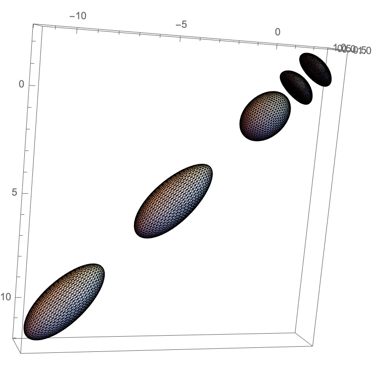 |
Compute the shape of a sphere centered at (2,2,2) in the moving reference system and moving with a speed of 0.5 in the positive x direction:
| In[4]:= |
| Out[4]= | 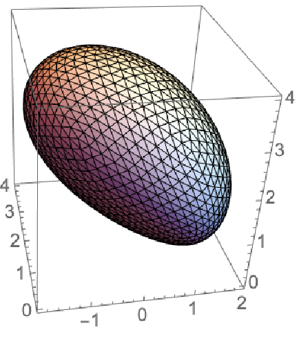 |
Show the observed shape of a cone initially positioned at (1,1,1), moving at a speed of 0.9 in the positive x direction:
| In[5]:= | ![Graphics3D[
ResourceFunction["RelativisticInertialDeformedRegion"][
Cone[], {1, 1, 1}, 0.9, Pi/2, Pi/2, 0, 1], Axes -> True]](https://www.wolframcloud.com/obj/resourcesystem/images/55e/55ed74f8-de0e-4441-9c14-f5b4fbcbc450/1ed2a941e5c52b46.png) |
| Out[5]= | 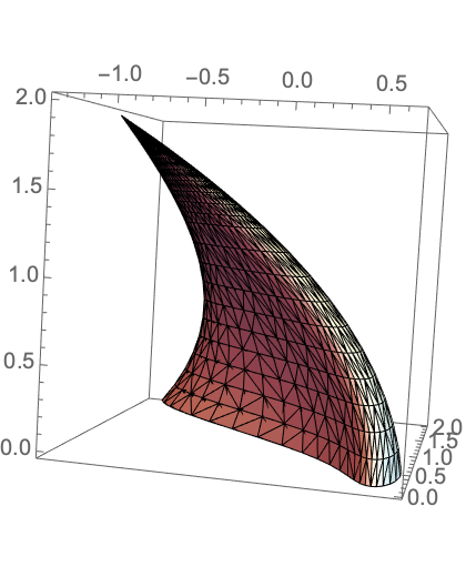 |
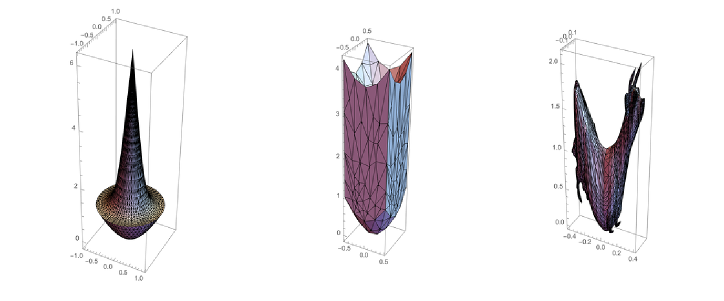
Simulate the visual appearance of different objects when traveling downwards with a speed of 0.95:
| In[6]:= | ![Table[Graphics3D[
ResourceFunction["RelativisticInertialDeformedRegion"][region, 0.95, \[Pi], \[Pi]/2, 0, 2000], Axes -> True], {region, {Cone[], Cube[], ExampleData[{"Geometry3D", "Cow"}, "Region"]}}]](https://www.wolframcloud.com/obj/resourcesystem/images/55e/55ed74f8-de0e-4441-9c14-f5b4fbcbc450/6585b4fe4c4d1108.png) |
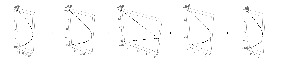
The shape of a vertical line at different times when moving in the x direction is a hyperbola, which degenerates to its asymptotes at time 0:
| In[7]:= | ![Table[Graphics3D[
ResourceFunction["RelativisticInertialDeformedRegion"][
Line[{{0, 0, -10}, {0, 0, 10}}], 0.9, time, 1], Axes -> True], {time, -6, 6, 3}]](https://www.wolframcloud.com/obj/resourcesystem/images/55e/55ed74f8-de0e-4441-9c14-f5b4fbcbc450/4e81b4873901022c.png) |
Show an icosahedron traveling with different speeds, observed at time 0:
| In[8]:= | ![Table[Graphics3D[
ResourceFunction["RelativisticInertialDeformedRegion"][
Icosahedron[], speed, 0, 3000], Axes -> True], {speed, 0.1, 0.9, 0.2}]](https://www.wolframcloud.com/obj/resourcesystem/images/55e/55ed74f8-de0e-4441-9c14-f5b4fbcbc450/7bdcde6242dc6dea.png) |
| In[9]:= | ![(* Evaluate this cell to get the example input *) CloudGet["https://www.wolframcloud.com/obj/b7526668-6455-4df1-8f27-8f96adca0d52"]](https://www.wolframcloud.com/obj/resourcesystem/images/55e/55ed74f8-de0e-4441-9c14-f5b4fbcbc450/4ecae10c01f809ea.png) |
We can also find the apparent shape of an implicit region:
| In[10]:= |
Show the shape of this region traveling upwards with a velocity of 0.8 at different times:
| In[11]:= |
| Out[11]= | 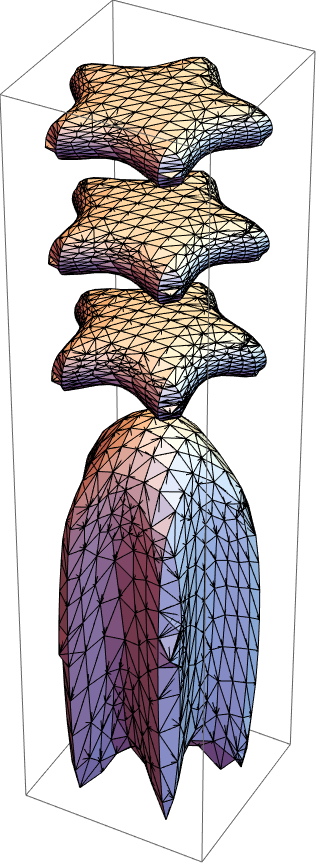 |
Show a torus moving at different speeds. Note that the centroid approaches the left edge of the torus as the speed increases:
| In[12]:= | ![Table[Show[
ResourceFunction["RelativisticInertialDeformedRegion"][
ExampleData[{"Geometry3D", "Torus"}, "Region"], speed, 0, 1], Graphics3D[{Red, PointSize[0.1], Point[RegionCentroid[
ResourceFunction["RelativisticInertialDeformedRegion"][
ExampleData[{"Geometry3D", "Torus"}, "Region"], speed, 0, 1]]]}] ], {speed, {0.2, 0.7, 0.9, 0.99, 0.99}}]](https://www.wolframcloud.com/obj/resourcesystem/images/55e/55ed74f8-de0e-4441-9c14-f5b4fbcbc450/20441351ebf85558.png) |
| Out[12]= | 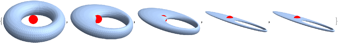 |
Plot the apparent length of a horizontal line versus time, when moving with a speed of 0.9 along the positive x-axis:
| In[13]:= | ![ListLinePlot[ AssociationThread[Subdivide[-10, 10, 20], Table[ArcLength[
ResourceFunction["RelativisticInertialDeformedRegion"][
Line[{{2, 0, 0}, {-2, 0, 0}}], 0.9, time, 10]], {time, -10, 10, 1}] ] ]](https://www.wolframcloud.com/obj/resourcesystem/images/55e/55ed74f8-de0e-4441-9c14-f5b4fbcbc450/64ed20329e9169e7.png) |
| Out[13]= | 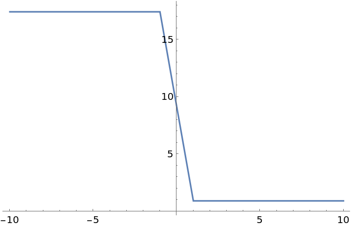 |
Use a vertical line:
| In[14]:= | ![ListLinePlot[ AssociationThread[Subdivide[-10, 10, 40], Table[ArcLength[
ResourceFunction["RelativisticInertialDeformedRegion"][
Line[{{0, 0, -2}, {0, 0, 2}}], 0.9, time, 10]], {time, -10, 10, 0.5}] ] , PlotRange -> All]](https://www.wolframcloud.com/obj/resourcesystem/images/55e/55ed74f8-de0e-4441-9c14-f5b4fbcbc450/7f2398491fddddc1.png) |
| Out[14]= | 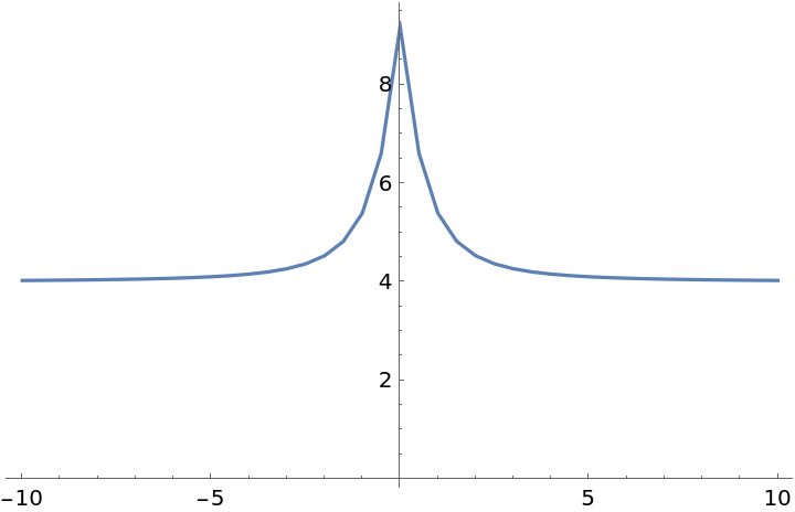 |
For some objects a higher accuracy goal may not work. For example, setting an accuracyGoal above 400 for the Wolfram Spikey leads to Mathematica running the code forever.
This work is licensed under a Creative Commons Attribution 4.0 International License