Wolfram Function Repository
Instant-use add-on functions for the Wolfram Language
Function Repository Resource:
Numerically estimate the limit of a sequence of values
ResourceFunction["SequenceLimit"][{n1,n2,…}] estimates the limit of the numerical sequence ni. |
| "WynnEpsilon" | top-level implementation of the Wynn epsilon algorithm |
| "NSequenceLimit" | built-in implementation of the Wynn epsilon algorithm from NumericalMath` |
| "BrezinskiTheta" | Brezinski's theta algorithm |
| "Euler" | Euler transformation |
| Automatic | chooses the method depending on the precision and length of the sequence |
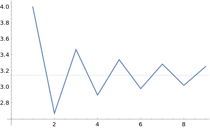
Build a sequence approximating Pi:
| In[1]:= |
|
| Out[1]= |
|
| In[2]:= |
|
| Out[2]= |
|
Find an approximation of the limit of the sequence:
| In[3]:= |
|
| Out[3]= |
|
The approximation is much closer to the limit than the last term of the sequence:
| In[4]:= |
|
| Out[4]= |
|
Symbolic sequences:
| In[5]:= |
|
| Out[5]= |
|
Rational sequences:
| In[6]:= |
|
| Out[6]= |
|
| In[7]:= |
|
| Out[7]= |
|
| In[8]:= |
|
| Out[8]= |
|
Real-valued sequences:
| In[9]:= |
|
| Out[9]= |
|
Complex-valued sequences:
| In[10]:= |
|
| Out[10]= |
|
| In[11]:= |
|
| Out[11]= |
|
Use the top-level implementation of the Wynn epsilon method:
| In[12]:= |
|
| Out[12]= |
|
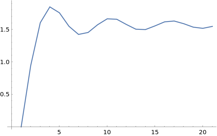
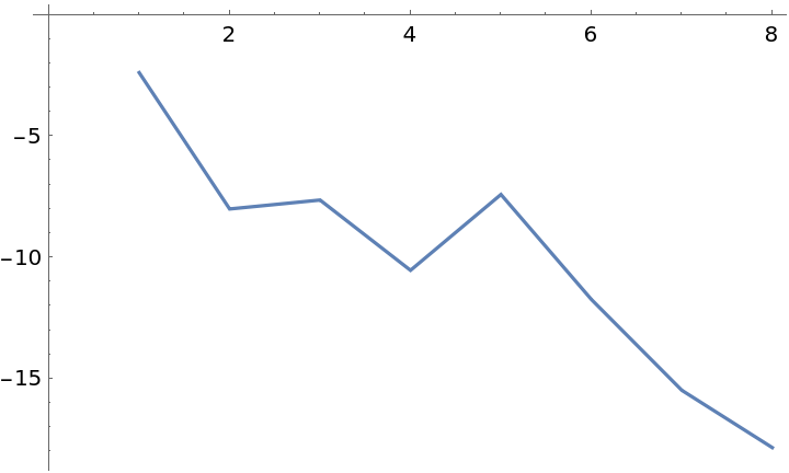
The top-level "WynnEpsilon" method can be more accurate:
| In[13]:= |
|
| In[14]:= |
|
| In[15]:= |
![ListPlot[Table[
Log@Abs[Pi/4 - Table[ResourceFunction["SequenceLimit"][pi4[n], Method -> method], {n, 5, 100}]], {method, methods}], Joined -> True, PlotLegends -> methods]](https://www.wolframcloud.com/obj/resourcesystem/images/542/542ee9e2-c30b-4452-857e-275a2d06e408/754ba8b429292c73.png)
|
| Out[15]= |

|
Generate partial sums of the Basel series:
| In[16]:= |
|
| Out[16]= |

|
With the default settings, "WynnEpsilon" does not give a good result:
| In[17]:= |
|
| Out[17]= |
|
Adjust the parameter of the transformation to give a better result:
| In[18]:= |
|
| Out[18]= |
|
| In[19]:= |
|
| Out[19]= |
|
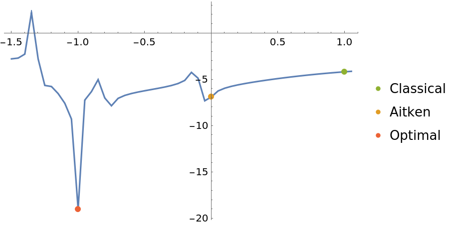
Plot the relative accuracy of the transformation for various values of the parameter:
| In[20]:= |
![Legended[ListLinePlot[
Table[{p, Log[Abs[ResourceFunction["SequenceLimit"][seq, Method -> {"WynnEpsilon", "Parameter" -> p}] - \[Pi]^2/
6]/(\[Pi]^2/6)]}, {p, -1.5, 1.05, 0.05}], Mesh -> {{{1, Directive[ColorData[97, 3], AbsolutePointSize[6]]}, {0, Directive[ColorData[97, 2], AbsolutePointSize[6]]}, {-1, Directive[ColorData[97, 4], AbsolutePointSize[6]]}}}, PlotRange -> All], PointLegend[{ColorData[97, 3], ColorData[97, 2], ColorData[97, 4]}, {"Classical", "Aitken", "Optimal"}]]](https://www.wolframcloud.com/obj/resourcesystem/images/542/542ee9e2-c30b-4452-857e-275a2d06e408/25ee00df213e1af2.png)
|
| Out[20]= |
|
Use the built-in implementation of the Wynn epsilon method:
| In[21]:= |
|
| Out[21]= |
|
Find approximations of the limit of a sequence using different Wynn degrees:
| In[22]:= |
|
| In[23]:= |
|
| Out[23]= |
|
| In[24]:= |
|
| Out[24]= |
|
Compare the errors:
| In[25]:= |
|
| Out[25]= |
|
| In[26]:= |
|
| Out[26]= |
|
The built-in "NSequenceLimit" method can be faster than the top-level implementation:
| In[27]:= |
|
| In[28]:= |
![RepeatedTiming[
Pi/4 - ResourceFunction["SequenceLimit"][seq, Method -> #]] & /@ {"WynnEpsilon", "NSequenceLimit"}](https://www.wolframcloud.com/obj/resourcesystem/images/542/542ee9e2-c30b-4452-857e-275a2d06e408/04073df7f053e39a.png)
|
| Out[28]= |
|
Partial sums of the :
| In[29]:= |
|
| Out[29]= |
|
Apply Brezinski's ϑ-algorithm to accelerate the convergence:
| In[30]:= |
|
| Out[30]= |
|
Compare with the exact result:
| In[31]:= |
|
| Out[31]= |
|
Partial sums of a Dirichlet series:
| In[32]:= |
|
| Out[32]= |
|
The Euler transformation gives better results than the default:
| In[33]:= |
|
| Out[33]= |
|
| In[34]:= |
|
| Out[34]= |
|
| In[35]:= |
|
| Out[35]= |
|
Partial sums of an alternating series:
| In[36]:= |
|
| Out[36]= |
|
Apply the Euler transformation:
| In[37]:= |
|
| Out[37]= |
|
Apply the Euler transformation with a different setting of the fixed ratio:
| In[38]:= |
|
| Out[38]= |
|
Compare both results with the exact result:
| In[39]:= |
|
| Out[39]= |
|
Applying SequenceLimit to the partial sums of a power series gives the same result as PadeApproximant:
| In[40]:= |
|
| In[41]:= |
|
| Out[41]= |

|
| In[42]:= |
![Block[{rat = Simplify[ResourceFunction["SequenceLimit"][ps]], c},
c = Coefficient[Denominator[rat], x, 0];
(Expand[Numerator[rat]/c])/(Expand[Denominator[rat]/c])]](https://www.wolframcloud.com/obj/resourcesystem/images/542/542ee9e2-c30b-4452-857e-275a2d06e408/3b556f388ba664eb.png)
|
| Out[42]= |

|
| In[43]:= |
|
| Out[43]= |

|
SequenceLimit can be used to compute limits, just like NLimit from NumericalCalculus`:
| In[44]:= |
|
| Out[44]= |
|
| In[45]:= |
|
| Out[45]= |
|
| In[46]:= |
|
| In[47]:= |
|
| Out[47]= |
|
SequenceLimit can encounter numerical errors:
| In[48]:= |
|
| Out[48]= |
|
| In[49]:= |
|
| Out[49]= |
|
Sometimes the errors can be avoided by numerically disturbing the sequence or changing its precision:
| In[50]:= |
|
| Out[50]= |
|
| In[51]:= |
|
| Out[51]= |
|
SequenceLimit can give unexpected results for divergent sequences:
| In[52]:= |
|
| Out[52]= |

|
| In[53]:= |
|
| Out[53]= |
|
| In[54]:= |
|
| Out[54]= |
|
This work is licensed under a Creative Commons Attribution 4.0 International License