Wolfram Function Repository
Instant-use add-on functions for the Wolfram Language
Function Repository Resource:
Compute the perpendicular surface of a curve
ResourceFunction["PerpendicularSurface"][c,t,{u,v},φ] computes the perpendicular surface with respect to variables u and v, making an angle ϕ with the normal surface of the curve parameterized by t. |
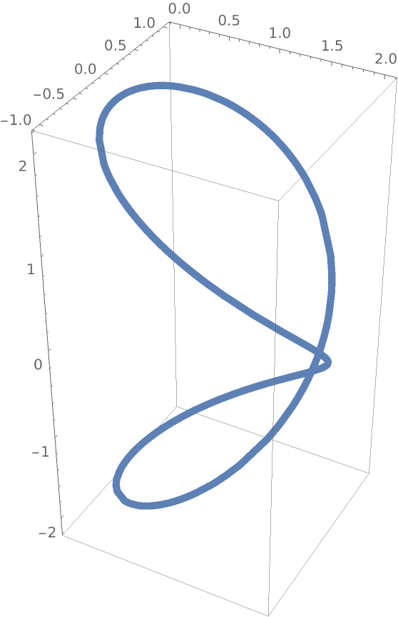
Viviani's curve:
| In[1]:= |
|
| Out[1]= |
|
Plot it:
| In[2]:= |
|
| Out[2]= |
|
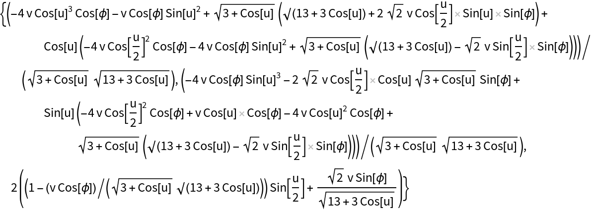
Compute the perpendicular surface for Viviani's curve:
| In[3]:= |
|
| Out[3]= |
|
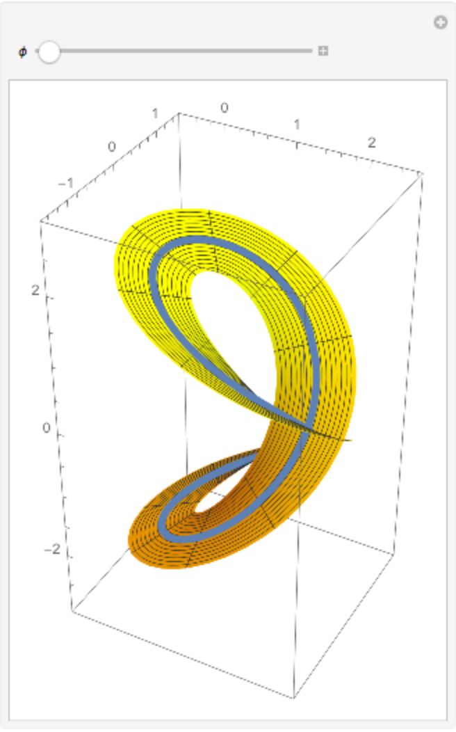
Plot both, varying the angle φ:
| In[4]:= |
![Manipulate[
Show[vp, ParametricPlot3D[
Evaluate[
ResourceFunction[
"PerpendicularSurface"][{1 + Cos[t], Sin[t], 2 Sin[t/2]}, t, {u, v}, \[Phi]]], {u, -2 \[Pi], 2 \[Pi]}, {v, -.5, .5}, PlotPoints -> {80, 10}, PlotStyle -> Yellow], PlotRange -> {{-0.5, 2.5}, {-1.4, 1.4}, {-2.7, 2.7}}], {\[Phi], 0, 2 \[Pi]}]](https://www.wolframcloud.com/obj/resourcesystem/images/4e3/4e3ac501-8398-4bfb-8c41-d798a548cf90/492683305a98ba75.png)
|
| Out[4]= |
|
The normal and binormal surfaces are special cases. Define Viviani's curve and compute its perpendicular surface:
| In[5]:= |
![viviani = Entity["SpaceCurve", "VivianiCurve"]["ParametricEquations"][1][t]
ResourceFunction[
"PerpendicularSurface"][{1 + Cos[t], Sin[t], 2 Sin[t/2]}, t, {u, v}, \[Phi]] - ResourceFunction["NormalSurface"][viviani, t, {u, v}] // Simplify](https://www.wolframcloud.com/obj/resourcesystem/images/4e3/4e3ac501-8398-4bfb-8c41-d798a548cf90/562542fb576e92b7.png)
|
| Out[5]= |
|
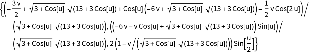
Compute the normal surface:
| In[6]:= |
|
| Out[6]= |
|
Compute the binormal surface:
| In[7]:= |
|
| Out[7]= |
|
Plots of normal and binormal surfaces:
| In[8]:= |
|
| In[9]:= |
|
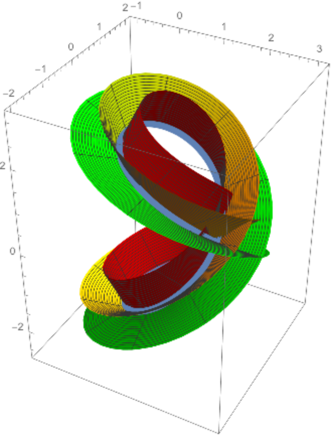
Combining the previous surfaces and Viviani's curve with an intermediate surface:
| In[10]:= |
![Show[vp, nsp, bsp, ParametricPlot3D[
Evaluate[ResourceFunction[
"PerpendicularSurface"][{1 + Cos[t], Sin[t], 2 Sin[t/2]}, t, {u, v}, 3 \[Pi]/4]], {u, -2 \[Pi], 2 \[Pi]}, {v, .05, 1}, PlotPoints -> {80, 10}, PlotStyle -> Yellow]]](https://www.wolframcloud.com/obj/resourcesystem/images/4e3/4e3ac501-8398-4bfb-8c41-d798a548cf90/7de918da61d55d99.png)
|
| Out[10]= |
|
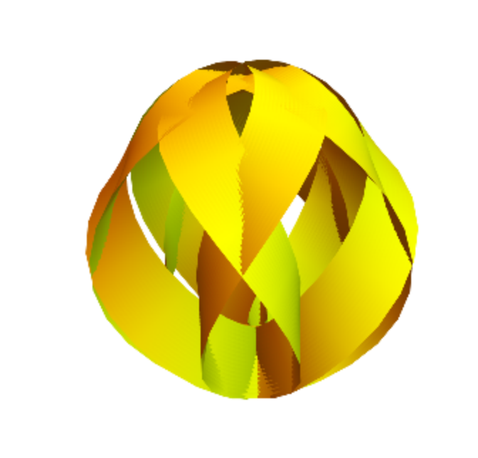
Perpendicular surface for the spherical spiral:
| In[11]:= |
![With[{a = 1, m = 3, n = 5}, ParametricPlot3D[
Evaluate[ResourceFunction[
"PerpendicularSurface"][{a Cos[m t] Cos[n t], a Sin[m t] Cos[n t],
a Sin[n t]}, t, {u, v}, 1]], {u, -2 \[Pi], 2 \[Pi]}, {v, -.25, .25}, PlotPoints -> {80, 10}, PlotStyle -> Yellow, Axes -> False, Boxed -> False, Mesh -> None]]](https://www.wolframcloud.com/obj/resourcesystem/images/4e3/4e3ac501-8398-4bfb-8c41-d798a548cf90/6b437a84142751e8.png)
|
| Out[11]= |
|
This work is licensed under a Creative Commons Attribution 4.0 International License