Wolfram Function Repository
Instant-use add-on functions for the Wolfram Language
Function Repository Resource:
Decompose a Riemannian or pseudo-Riemannian manifold into a union of discrete hypersurfaces
ResourceFunction["DiscreteHypersurfaceDecomposition"][MetricTensor[…],{t,tinit,tfinal},{x,xmin,xmax},{y,ymin,ymax},n,disc] represents the decomposition of the given MetricTensor into generalized "spacelike" hypersurfaces with "spatial" coordinates x and y, and "time" coordinate t, using n points for the discretization, and with a discreteness scale of disc. | |
ResourceFunction["DiscreteHypersurfaceDecomposition"][MetricTensor[…],{t,tinit,tfinal},{x,xmin,xmax},{y,ymin,ymax}] uses 100 points for the discretization and assumes a discreteness scale of 1. | |
ResourceFunction["DiscreteHypersurfaceDecomposition"][MetricTensor[…],…,n,disc] uses the first coordinate of the MetricTensor as the "time" coordinate, and the second and third coordinate of the MetricTensor as the "spatial" coordinates. | |
ResourceFunction["DiscreteHypersurfaceDecomposition"][ResourceFunction["DiscreteHypersurfaceDecomposition"][…],coords] transforms a specified ResourceFunction["DiscreteHypersurfaceDecomposition"] into the new coordinate system coords. |
| "CoordinatizedPolarGraphColored" | final hypersurface of the decomposition in polar coordinates, represented as an undirected graph with vertices colored based on (extrinsic) curvature and with spatial coordinates assigned based on hypersurface embedding information |
| "PolarGraphColored" | final hypersurface of the decomposition in polar coordinates, represented as an undirected graph with vertices colored based on (extrinsic) curvature |
| "CoordinatizedPolarGraph" | final hypersurface of the decomposition in polar coordinates, represented as an undirected graph with spatial coordinates of vertices assigned based on hypersurface embedding information |
| "PolarGraph" | final hypersurface of the decomposition in polar coordinates, represented as an undirected graph |
| "CoordinatizedPolarGraphEvolutionColored" | list of 10 hypersurfaces (plus initial data) representing the full "evolution history" of the decomposition in polar coordinates, represented as undirected graphs with vertices colored based on (extrinsic) curvature and with spatial coordinates assigned based on hypersurface embedding information |
| {"CoordinatizedPolarGraphEvolutionColored",steps} | list of steps hypersurfaces (plus initial data) representing the full "evolution history" of the decomposition in polar coordinates, represented as undirected graphs with vertices colored based on (extrinsic) curvature and with spatial coordinates assigned based on hypersurface embedding information |
| "PolarGraphEvolutionColored" | list of 10 hypersurfaces (plus initial data) representing the full "evolution history" of the decomposition in polar coordinates, represented as undirected graphs with vertices colored based on (extrinsic) curvature |
| {"PolarGraphEvolutionColored",steps} | list of steps hypersurfaces (plus initial data) representing the full "evolution history" of the decomposition in polar coordinates, represented as undirected graphs with vertices colored based on (extrinsic) curvature |
| "CoordinatizedPolarGraphEvolution" | list of 10 hypersurfaces (plus initial data) representing the full "evolution history" of the decomposition in polar coordinates, represented as undirected graphs with spatial coordinates of vertices assigned based on hypersurface embedding information |
| {"CoordinatizedPolarGraphEvolution",steps} | list of steps hypersurfaces (plus initial data) representing the full "evolution history" of the decomposition in polar coordinates, represented as undirected graphs with spatial coordinates of vertices assigned based on hypersurface embedding information |
| "PolarGraphEvolution" | list of 10 hypersurfaces (plus initial data) representing the full "evolution history" of the decomposition in polar coordinates, represented as undirected graphs |
| {"PolarGraphEvolution",steps} | list of steps hypersurfaces (plus initial data) representing the full "evolution history" of the decomposition in polar coordinates, represented as undirected graphs |
| "CoordinatizedCartesianGraphColored" | final hypersurface of the decomposition in Cartesian coordinates, represented as an undirected graph with vertices colored based on (extrinsic) curvature and with spatial coordinates assigned based on hypersurface embedding information |
| "CartesianGraphColored" | final hypersurface of the decomposition in Cartesian coordinates, represented as an undirected graph with vertices colored based on (extrinsic) curvature |
| "CoordinatizedCartesianGraph" | final hypersurface of the decomposition in Cartesian coordinates, represented as an undirected graph with spatial coordinates of vertices assigned based on hypersurface embedding information |
| "CartesianGraph" | final hypersurface of the decomposition in Cartesian coordinates, represented as an undirected graph |
| "CoordinatizedCartesianGraphEvolutionColored" | list of 10 hypersurfaces (plus initial data) representing the full "evolution history" of the decomposition in Cartesian coordinates, represented as undirected graphs with vertices colored based on (extrinsic) curvature and with spatial coordinates assigned based on hypersurface embedding information |
| {"CoordinatizedCartesianGraphEvolutionColored",steps} | list of steps hypersurfaces (plus initial data) representing the full "evolution history" of the decomposition in Cartesian coordinates, represented as undirected graphs with vertices colored based on (extrinsic) curvature and with spatial coordinates assigned based on hypersurface embedding information |
| "CartesianGraphEvolutionColored" | list of 10 hypersurfaces (plus initial data) representing the full "evolution history" of the decomposition in Cartesian coordinates, represented as undirected graphs with vertices colored based on (extrinsic) curvature |
| {"CartesianGraphEvolutionColored",steps} | list of steps hypersurfaces (plus initial data) representing the full "evolution history" of the decomposition in Cartesian coordinates, represented as undirected graphs with vertices colored based on (extrinsic) curvature |
| "CoordinatizedCartesianGraphEvolution" | list of 10 hypersurfaces (plus initial data) representing the full "evolution history" of the decomposition in Cartesian coordinates, represented as undirected graphs with spatial coordinates of vertices assigned based on hypersurface embedding information |
| {"CoordinatizedCartesianGraphEvolution",steps} | list of steps hypersurfaces (plus initial data) representing the full "evolution history" of the decomposition in Cartesian coordinates, represented as undirected graphs with spatial coordinates of vertices assigned based on hypersurface embedding information |
| "CartesianGraphEvolution" | list of 10 hypersurfaces (plus initial data) representing the full "evolution history" of the decomposition in Cartesian coordinates, represented as undirected graphs |
| {"CartesianGraphEvolution",steps} | list of steps hypersurfaces (plus initial data) representing the full "evolution history" of the decomposition in Cartesian coordinates, represented as undirected graphs |
| "MetricTensor" | underlying metric tensor associated to the discrete hypersurface decomposition |
| "Coordinates" | list of coordinate symbols for the discrete hypersurface decomposition |
| "CoordinateOneForms" | list of differential 1-form symbols for the coordinates of the discrete hypersurface decomposition |
| "TimeCoordinate" | distinguished "time" coordinate symbol for the discrete hypersurface decomposition |
| "TimeInterval" | 1-dimensional interval (range) of the distinguished "time" coordinate for the discrete hypersurface decomposition |
| "SpatialCoordinates" | distinguished "spatial" coordinate symbols for the discrete hypersurface decomposition |
| "SpatialRegion" | 2-dimensional region (range) of the distinguished "spatial" coordinates for the discrete hypersurface decomposition |
| "VertexCount" | number of points (vertices) in each discrete hypersurface of the decomposition |
| "DiscretizationScale" | discretization scale for each discrete hypersurface of the decomposition |
| "Dimensions" | number of dimensions of the underlying manifold/spacetime described by the discrete hypersurface decomposition |
| "Signature" | list of +1s and -1s designating the signature of the underlying manifold described by the discrete hypersurface decomposition (+1 for each positive eigenvalue of the metric, -1 for each negative eigenvalue of the metric) |
| "RiemannianQ" | whether the underlying manifold described by the discrete hypersurface decomposition is Riemannian (i.e. all eigenvalues of the metric have the same sign) |
| "PseudoRiemannianQ" | whether the underlying manifold described by the discrete hypersurface decomposition is pseudo-Riemannian (i.e. all eigenvalues of the metric are non-zero, but not all have the same sign) |
| "LorentzianQ" | whether the underlying manifold described by the discrete hypersurface decomposition is Lorentzian (i.e. all eigenvalues of the metric have the same sign, except for one eigenvalue which has the opposite sign) |
| "RiemannianConditions" | list of conditions required to guarantee that the underlying manifold described by the discrete hypersurface decomposition is Riemannian (i.e. all eigenvalues of the metric are positive) |
| "PseudoRiemannianConditions" | list of conditions required to guarantee that the underlying manifold described by the discrete hypersurface decomposition is pseudo-Riemannian (i.e. all eigenvalues of the metric are non-zero) |
| "LorentzianConditions" | list of conditions required to guarantee that the underlying manifold described by the discrete hypersurface decomposition is Lorentzian (i.e. the "time" eigenvalue of the metric is negative and all other eigenvalues are positive) |
| "Properties" | list of properties |
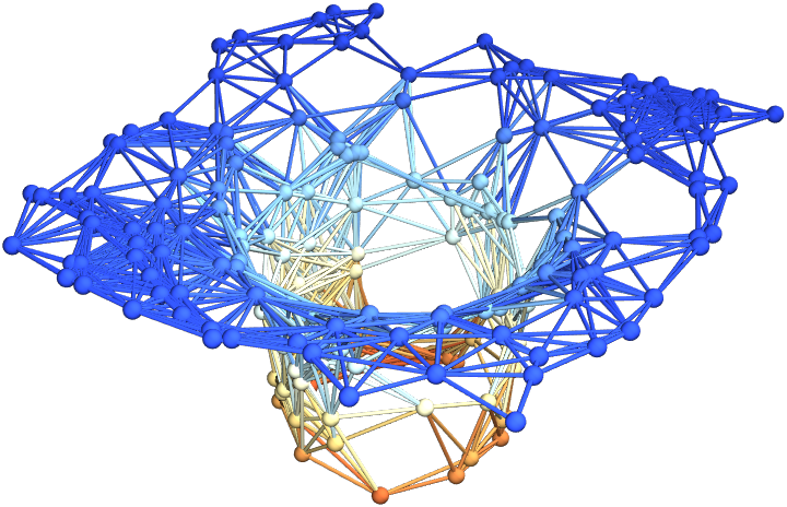
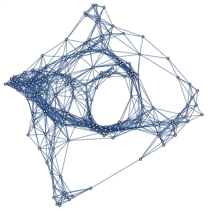
Construct a discrete hypersurface decomposition for the Schwarzschild metric (e.g. for an uncharged, non-rotating black hole with numerical mass 1) in standard spherical polar coordinates, with time coordinate t ranging between 0 and 1, radial coordinate r ranging between 0 and 4 and angular coordinate a1 ranging between -Pi and Pi, using 200 vertices and a discretization scale of 1.5:
| In[1]:= |
| Out[1]= |  |
| In[2]:= |
| Out[2]= |
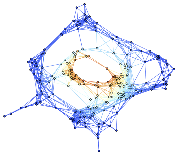
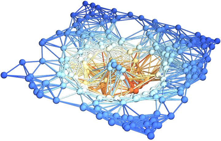
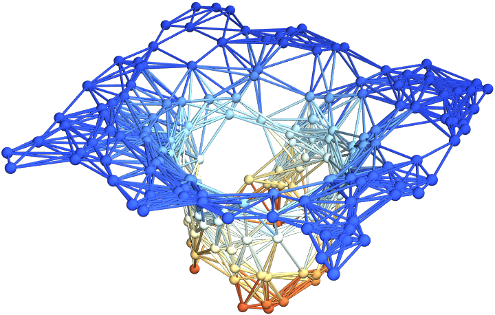
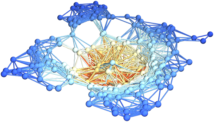
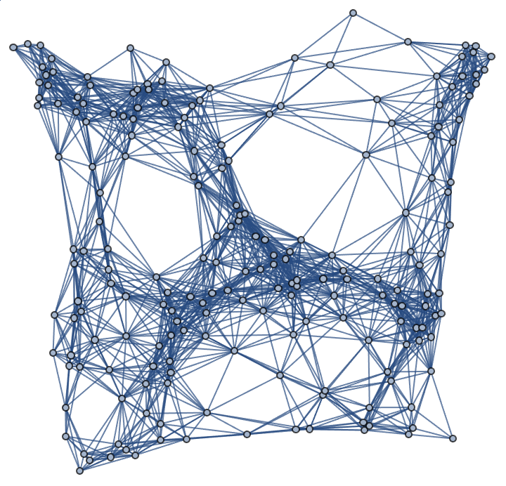
Show the final hypersurface of the decomposition in polar coordinates, with colors based on extrinsic curvature and spatial coordinates based on hypersurface embedding information:
| In[3]:= |
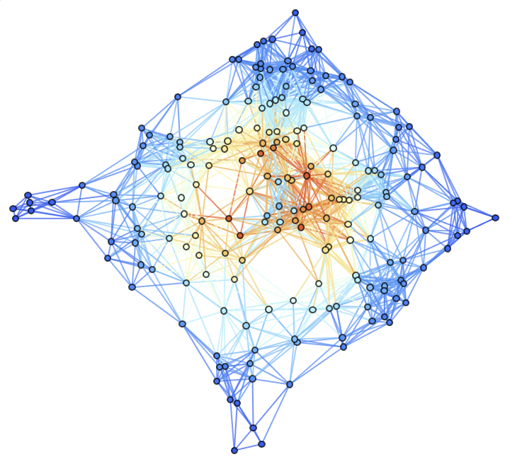
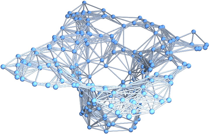
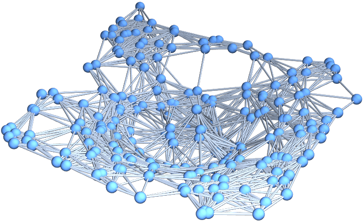
Show the final hypersurface of the decomposition in polar coordinates, with all spatial coordinate information removed:
| In[4]:= |
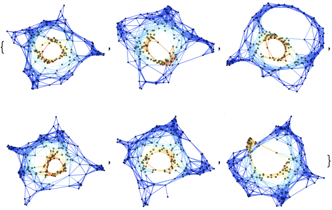
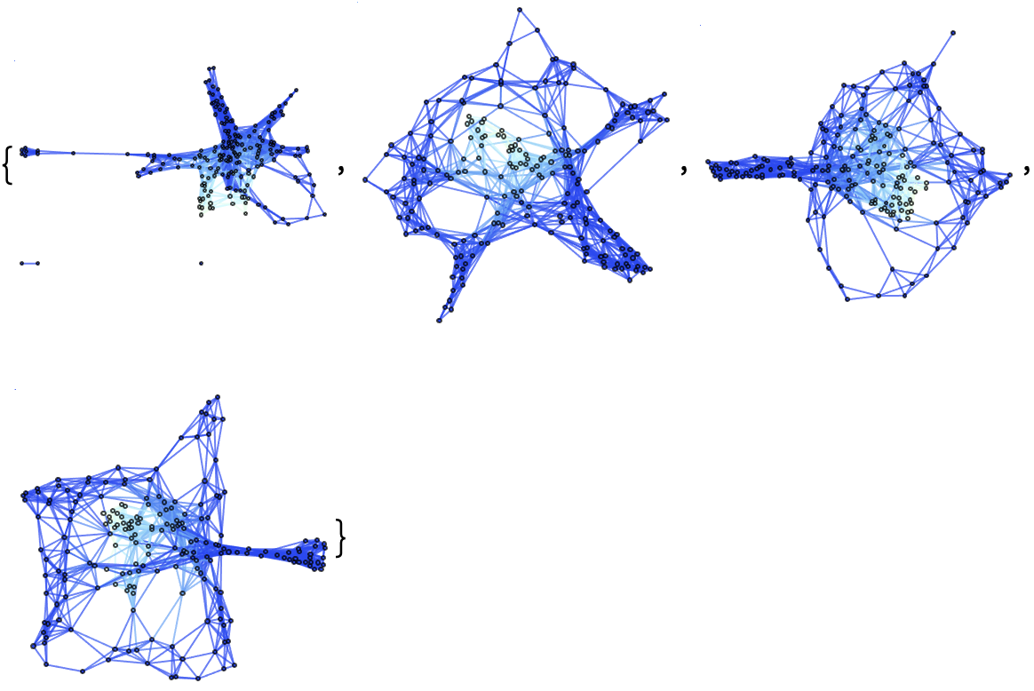
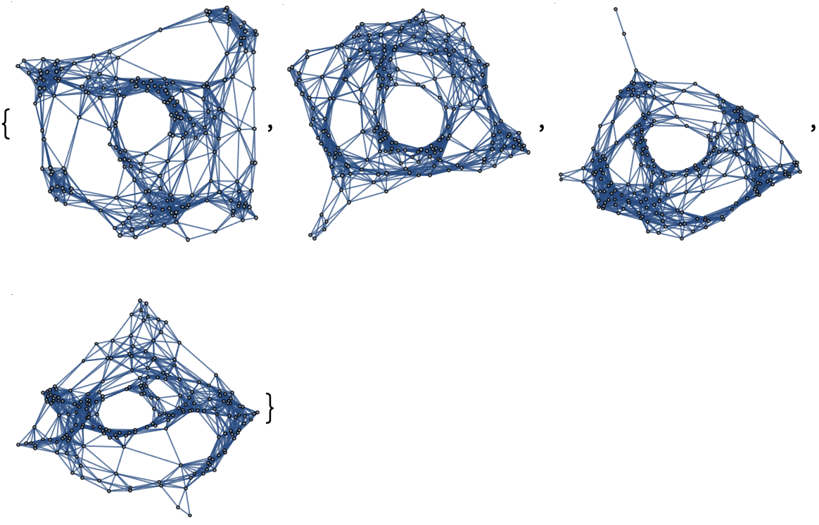
Show a list of 5 hypersurfaces (plus initial data) representing the complete "evolution" of the decomposition in polar coordinates, with colors based on extrinsic curvature:
| In[5]:= |
Construct a discrete hypersurface decomposition of the same (Schwarzschild) metric, but using 400 vertices and a discretization scale of 1 instead:
| In[6]:= |
| Out[6]= |
| In[7]:= |
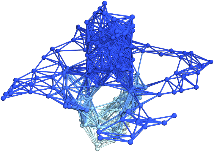
(Note that the remaining examples within this subsection are likely to require in excess of 1 minute of total computation time to evaluate on a typical personal computer.) Construct a discrete hypersurface decomposition of the same (Schwarzschild) metric in "Cartesian-like" isotropic coordinates, in which all light cones appear round, with time coordinate t still ranging between 0 and 1, x coordinate ranging between -2 and 2 and y coordinate ranging between -2 and 2, using 200 vertices and a discretization scale of 0.75:
| In[8]:= |
| Out[8]= |  |
| In[9]:= |
| Out[9]= |
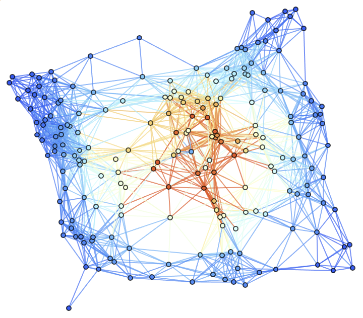
Show the final hypersurface of the decomposition in Cartesian coordinates, with colors based on extrinsic curvature and spatial coordinates based on hypersurface embedding information:
| In[10]:= |
Show the final hypersurface of the decomposition in Cartesian coordinates, with all spatial coordinate information removed:
| In[11]:= |
Construct a discrete hypersurface decomposition for the Kerr metric (e.g. for an uncharged, spinning black hole with numerical mass 1 and numerical angular momentum 1/3) in Boyer-Lindquist/oblate spheroidal coordinates, with time coordinate t ranging between 0 and 1, radial coordinate r ranging between 0 and 4 and angular coordinate a1 ranging between -Pi and Pi, using 200 vertices and a discretization scale of 1.5:
| In[12]:= |
| Out[12]= |  |
| In[13]:= |
| Out[13]= |
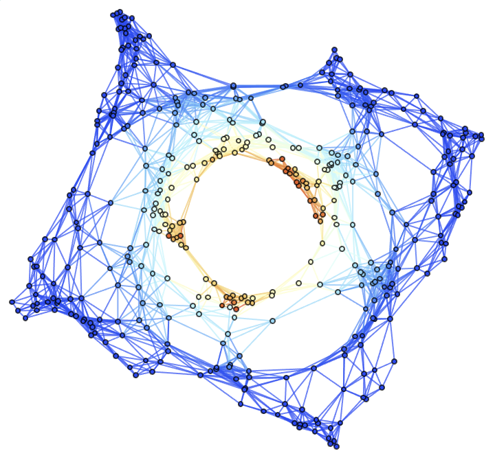
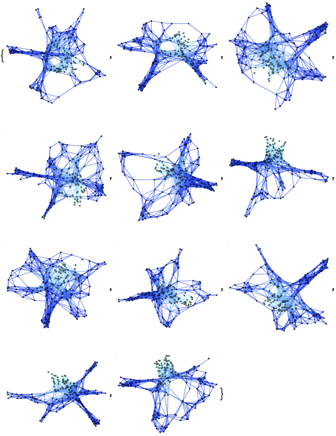
Show a list of 10 hypersurfaces (plus initial data) representing the complete "evolution" of the decomposition in polar coordinates, with colors based on extrinsic curvature and spatial coordinates based on hypersurface embedding information:
| In[14]:= |
(Note that the remaining examples within this subsection are likely to require in excess of 1 minute of total computation time to evaluate on a typical personal computer.) Show a list of 10 hypersurfaces (plus initial data) representing the complete "evolution" of the decomposition in polar coordinates, with all spatial coordinate information removed:
| In[15]:= |
Show a list of only 3 hypersurfaces (plus initial data) characterizing the evolution instead:
| In[16]:= |
If not otherwise specified, default values will be chosen for the vertex count n and the discretization scale disc (namely 100 and 1, respectively):
| In[17]:= | ![decomposition = ResourceFunction["DiscreteHypersurfaceDecomposition"][
ResourceFunction["MetricTensor"][{"Schwarzschild", 1}, {t, r, a1, a2}], {t, 0, 1}, {r, 0, 4}, {a1, -Pi, Pi}]](https://www.wolframcloud.com/obj/resourcesystem/images/4aa/4aadf4ae-5c48-42da-af9c-fc53e692377b/7b63d2232a2bbbfa.png) |
| Out[17]= |
| In[18]:= |
| Out[18]= |
| In[19]:= |
| Out[19]= |
Likewise for the time coordinate t and the spatial coordinates x and y (namely the first coordinate and the second and third coordinates of the underlying MetricTensor, respectively), along with their respective ranges:
| In[20]:= |
| Out[20]= |
| In[21]:= |
| Out[21]= |
| In[22]:= |
| Out[22]= |
| In[23]:= |
| Out[23]= |
| In[24]:= |
| Out[24]= |
Or for both simultaneously:
| In[25]:= |
| Out[25]= |
| In[26]:= |
| Out[26]= |
| In[27]:= |
| Out[27]= |
New coordinate symbols can be specified for any discrete hypersurface decomposition:
| In[28]:= |
| Out[28]= |
| In[29]:= |
| Out[29]= |
| In[30]:= |
| Out[30]= |
| In[31]:= |
| Out[31]= |
Construct a discrete hypersurface decomposition for the Reissner-Nordström metric (e.g. for a charged, non-rotating black hole with numerical mass 1 and numerical electric charge 1/2) in standard spherical polar coordinates, with time coordinate t ranging between 0 and 1, radial coordinate r ranging between 0 and 4 and angular coordinate a1 ranging between -Pi and Pi, using 200 vertices and a discretization scale of 1.5:
| In[32]:= |
| Out[32]= |  |
| In[33]:= |
| Out[33]= |
Show the list of properties:
| In[34]:= |
| Out[34]= |  |
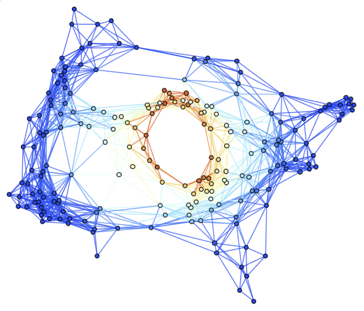
Show the final hypersurface of the decomposition in polar coordinates, with colors based on extrinsic curvature and spatial coordinates based on hypersurface embedding information:
| In[35]:= |
Show the final hypersurface of the decomposition in polar coordinates, with colors based on extrinsic curvature:
| In[36]:= |
Show the final hypersurface of the decomposition in polar coordinates, with spatial coordinates based on hypersurface embedding information:
| In[37]:= |
Show the final hypersurface of the decomposition in polar coordinates:
| In[38]:= |
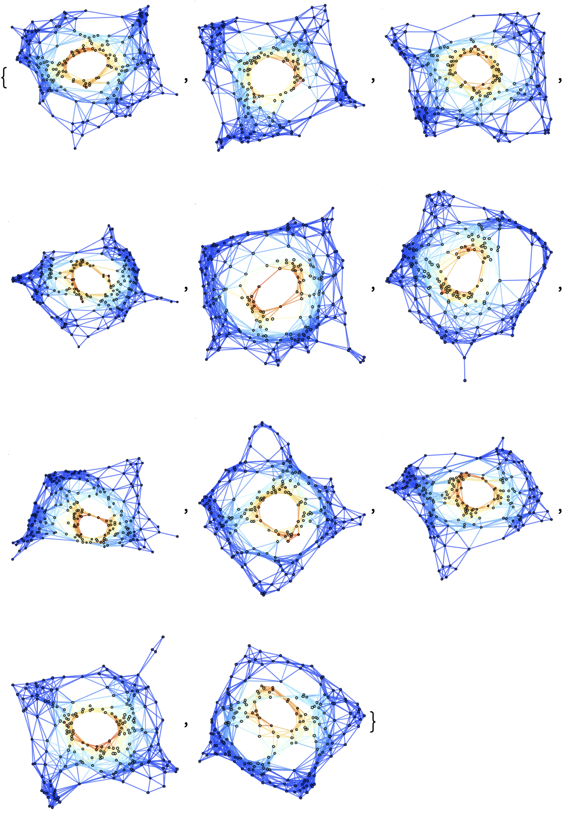
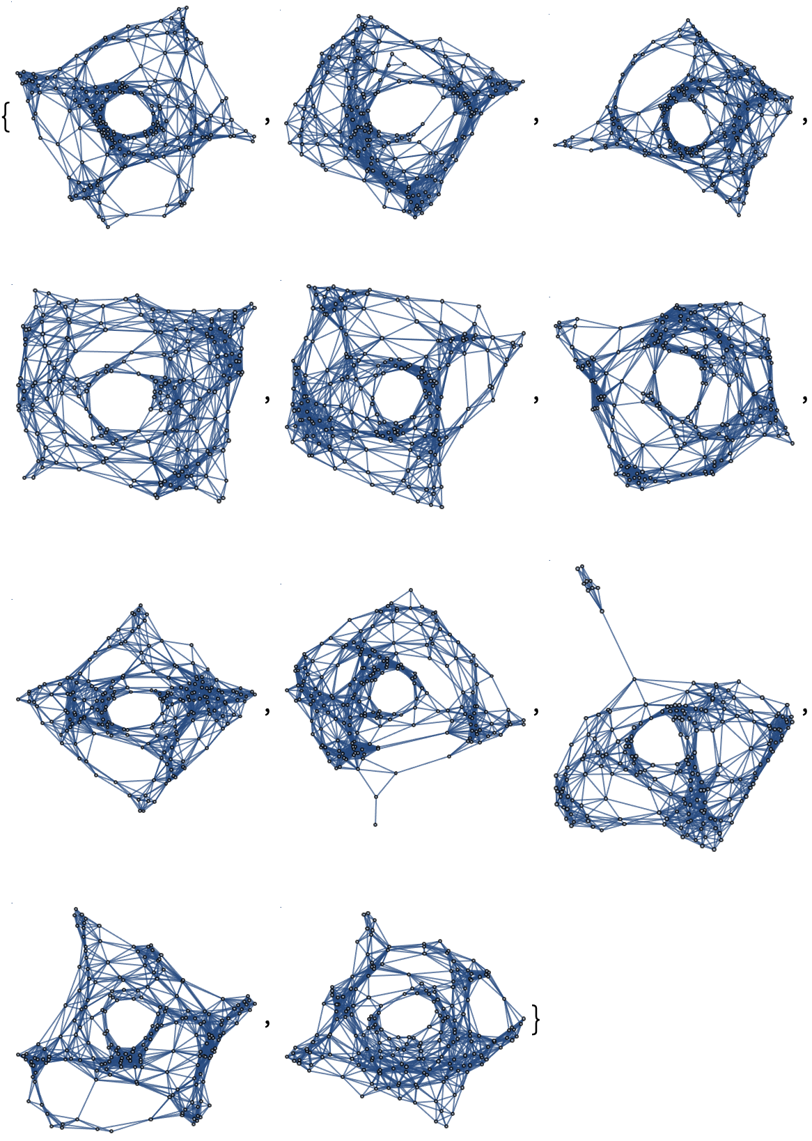
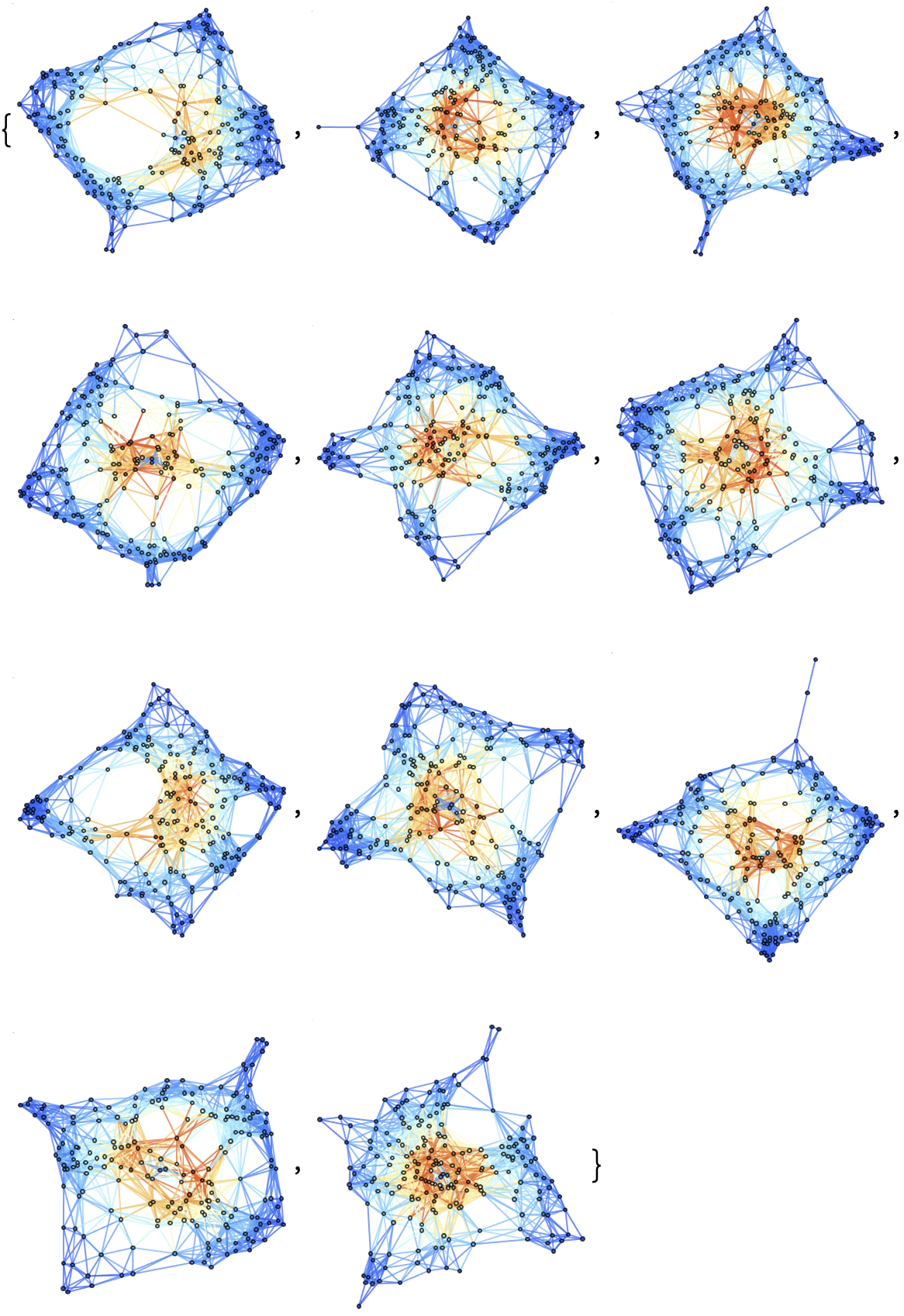
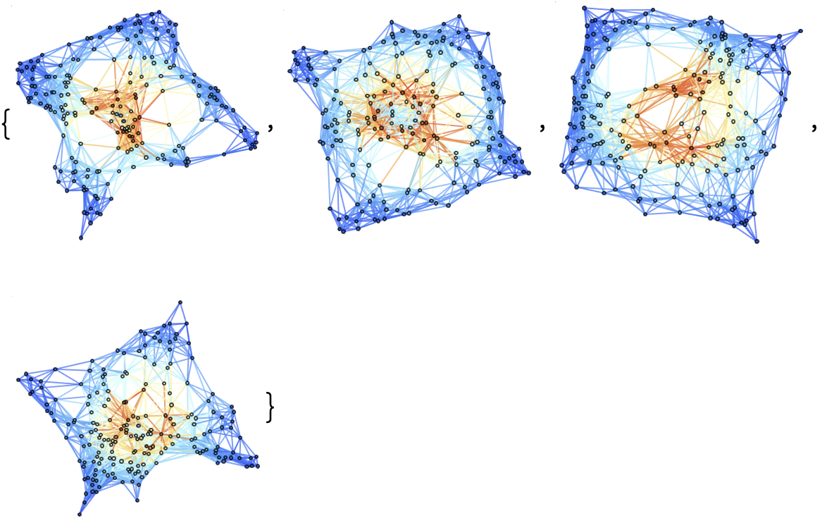
Show a list of 10 hypersurfaces (plus initial data) representing the complete "evolution" of the decomposition in polar coordinates, with colors based on extrinsic curvature and spatial coordinates based on hypersurface embedding information:
| In[39]:= |
| Out[39]= | 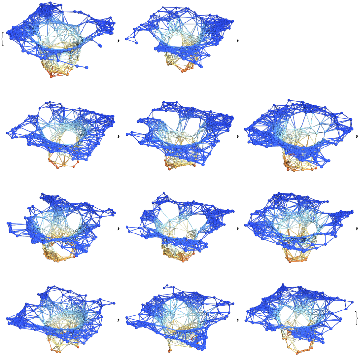 |
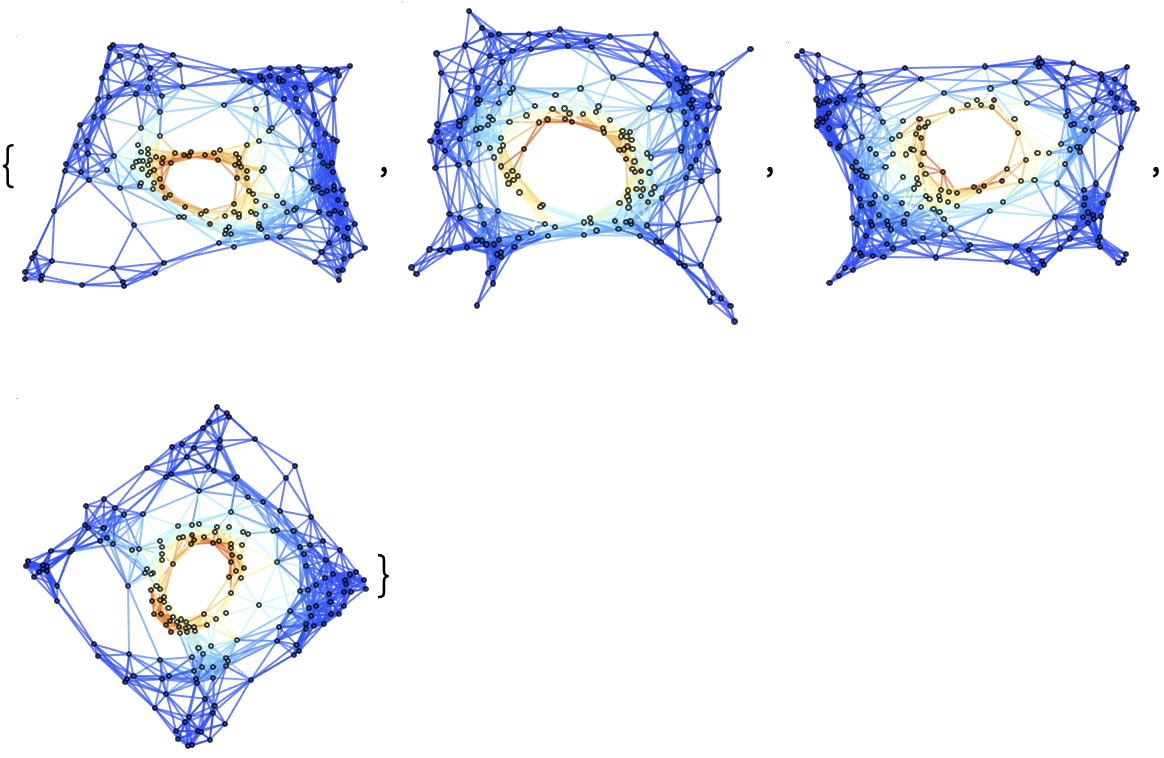
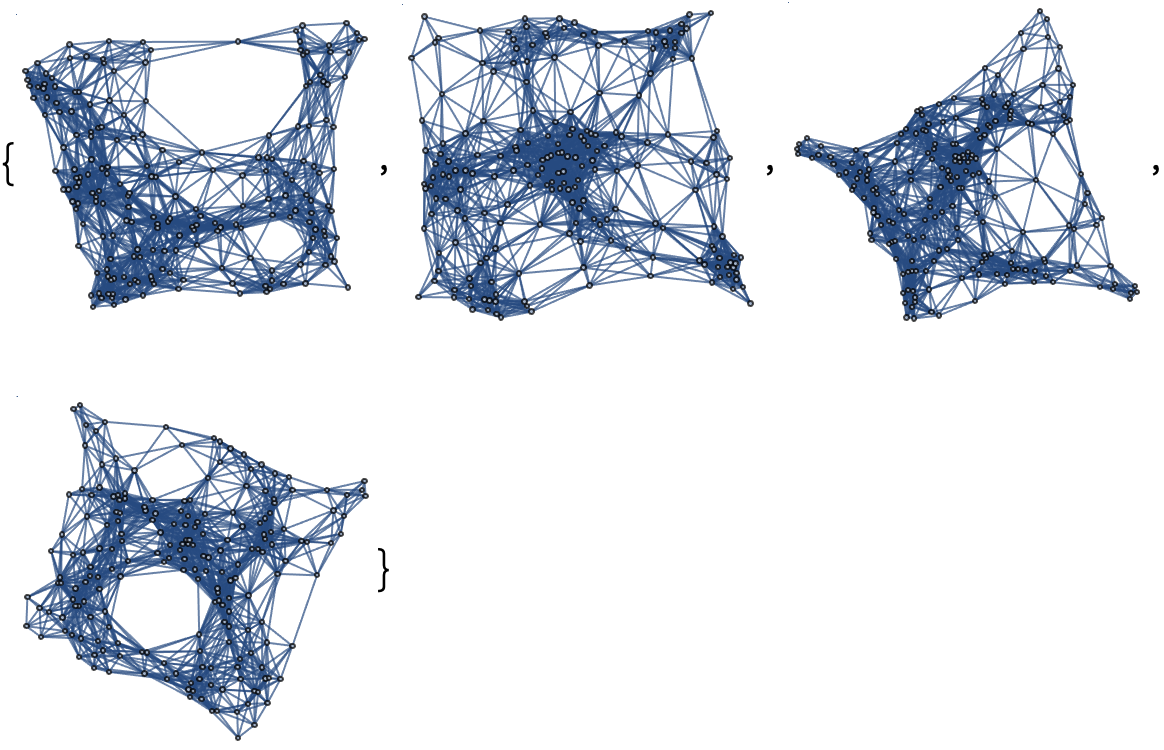
Show a list of 3 hypersurfaces (plus initial data) representing the complete "evolution" of the decomposition in polar coordinates, with colors based on extrinsic curvature and spatial coordinates based on hypersurface embedding information:
| In[40]:= |
| Out[40]= | 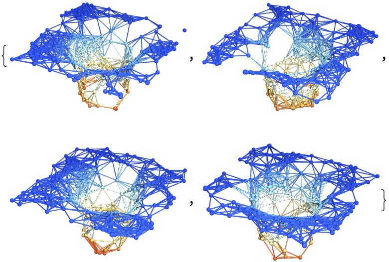 |
Show a list of 10 hypersurfaces (plus initial data) representing the complete "evolution" of the decomposition in polar coordinates, with colors based on extrinsic curvature:
| In[41]:= |
Show a list of 3 hypersurfaces (plus initial data) representing the complete "evolution" of the decomposition in polar coordinates, with colors based on extrinsic curvature:
| In[42]:= |
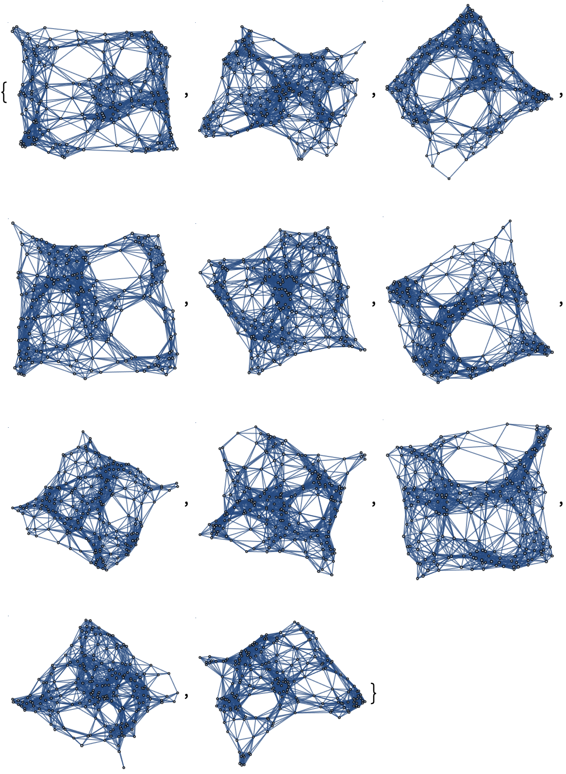
Show a list of 10 hypersurfaces (plus initial data) representing the complete "evolution" of the decomposition in polar coordinates, with spatial coordinates based on hypersurface embedding information:
| In[43]:= |
| Out[43]= | 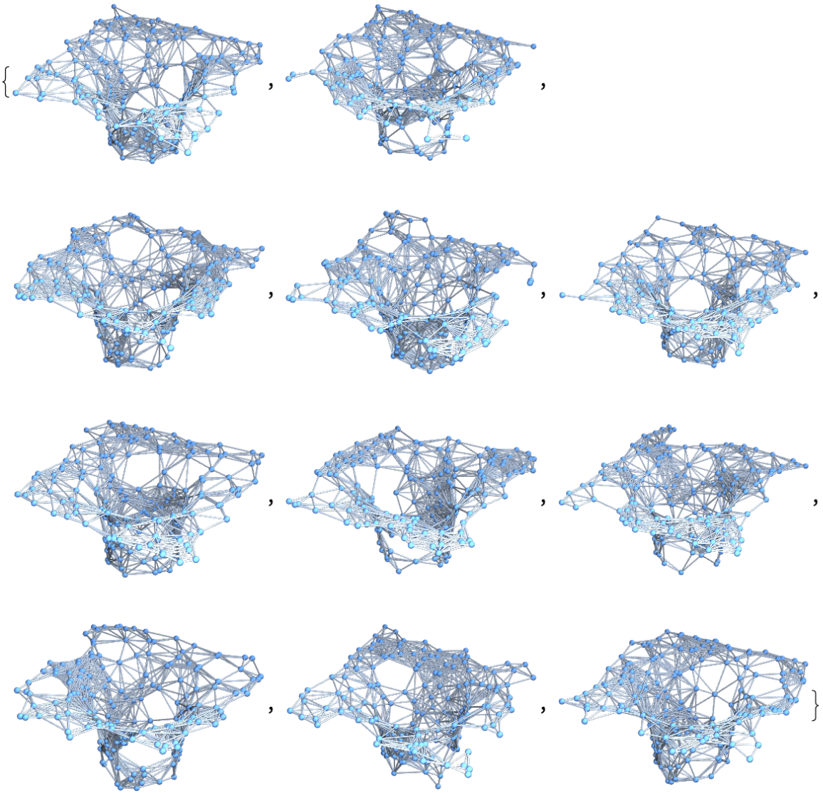 |
Show a list of 3 hypersurfaces (plus initial data) representing the complete "evolution" of the decomposition in polar coordinates, with spatial coordinates based on hypersurface embedding information:
| In[44]:= |
| Out[44]= | 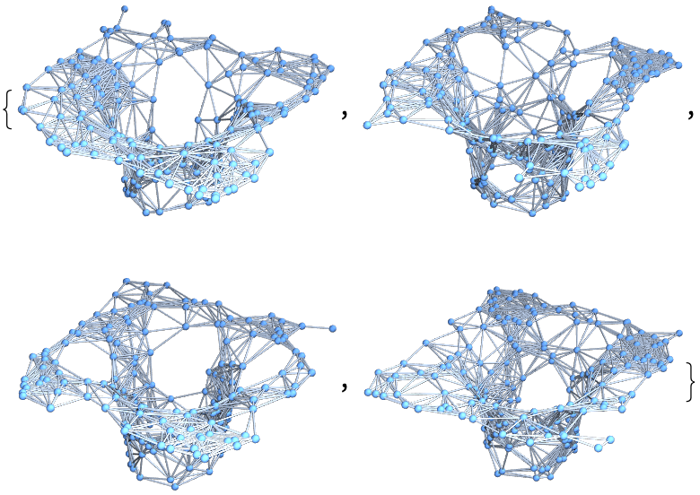 |
Show a list of 10 hypersurfaces (plus initial data) representing the complete "evolution" of the decomposition in polar coordinates:
| In[45]:= |
Show a list of 3 hypersurfaces (plus initial data) representing the complete "evolution" of the decomposition in polar coordinates:
| In[46]:= |
(Note that the remaining examples within this subsection are likely to require in excess of 1 minute of total computation time to evaluate on a typical personal computer.) Construct a discrete hypersurface decomposition of the Schwarzschild metric (e.g. for an uncharged, non-rotating black hole with numerical mass 1) in "Cartesian-like" isotropic coordinates, in which all light cones appear round, with time coordinate t still ranging between 0 and 1, x coordinate ranging between -2 and 2 and y coordinate ranging between -2 and 2, using 200 vertices and a discretization scale of 0.75:
| In[47]:= |
| Out[47]= |  |
| In[48]:= |
| Out[48]= |
Show the final hypersurface of the decomposition in Cartesian coordinates, with colors based on extrinsic curvature and spatial coordinates based on hypersurface embedding information:
| In[49]:= |
Show the final hypersurface of the decomposition in Cartesian coordinates, with colors based on extrinsic curvature:
| In[50]:= |
Show the final hypersurface of the decomposition in Cartesian coordinates, with spatial coordinates based on hypersurface embedding information:
| In[51]:= |
Show the final hypersurface of the decomposition in Cartesian coordinates:
| In[52]:= |
Show a list of 10 hypersurfaces (plus initial data) representing the complete "evolution" of the decomposition in Cartesian coordinates, with colors based on extrinsic curvature and spatial coordinates based on hypersurface embedding information:
| In[53]:= |
| Out[53]= | 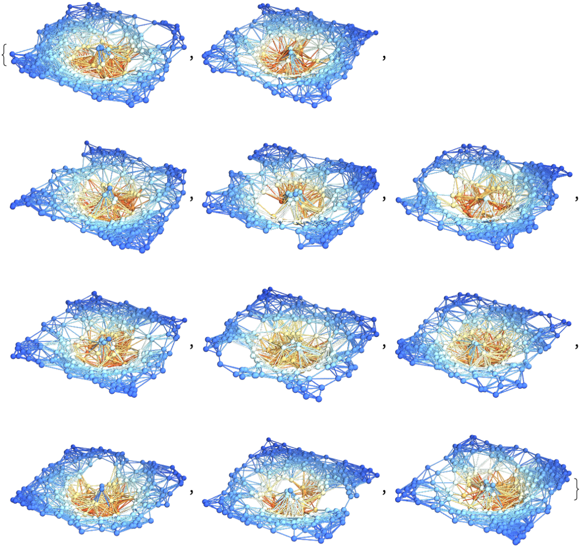 |
Show a list of 3 hypersurfaces (plus initial data) representing the complete "evolution" of the decomposition in Cartesian coordinates, with colors based on extrinsic curvature and spatial coordinates based on hypersurface embedding information:
| In[54]:= |
| Out[54]= | 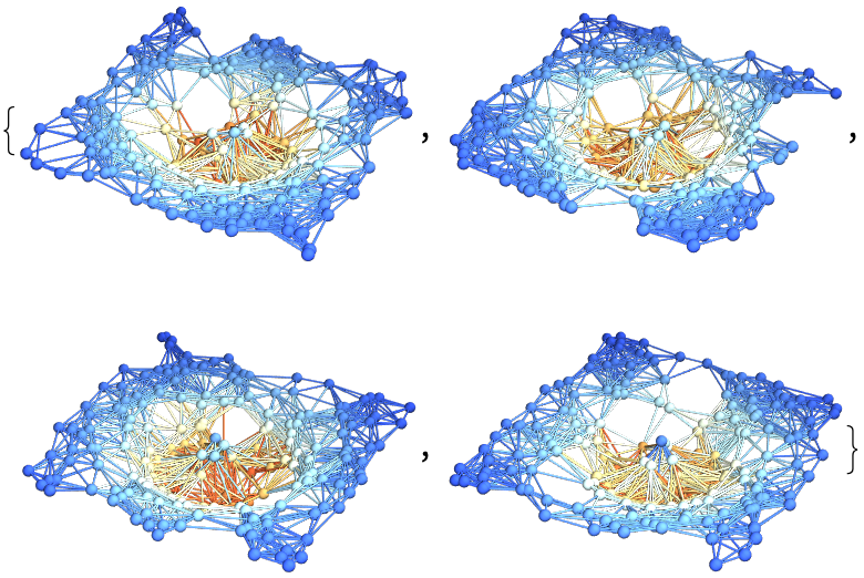 |
Show a list of 10 hypersurfaces (plus initial data) representing the complete "evolution" of the decomposition in Cartesian coordinates, with colors based on extrinsic curvature:
| In[55]:= |
Show a list of 3 hypersurfaces (plus initial data) representing the complete "evolution" of the decomposition in Cartesian coordinates, with colors based on extrinsic curvature:
| In[56]:= |
Show a list of 10 hypersurfaces (plus initial data) representing the complete "evolution" of the decomposition in Cartesian coordinates, with spatial coordinates based on hypersurface embedding information:
| In[57]:= |
| Out[57]= | 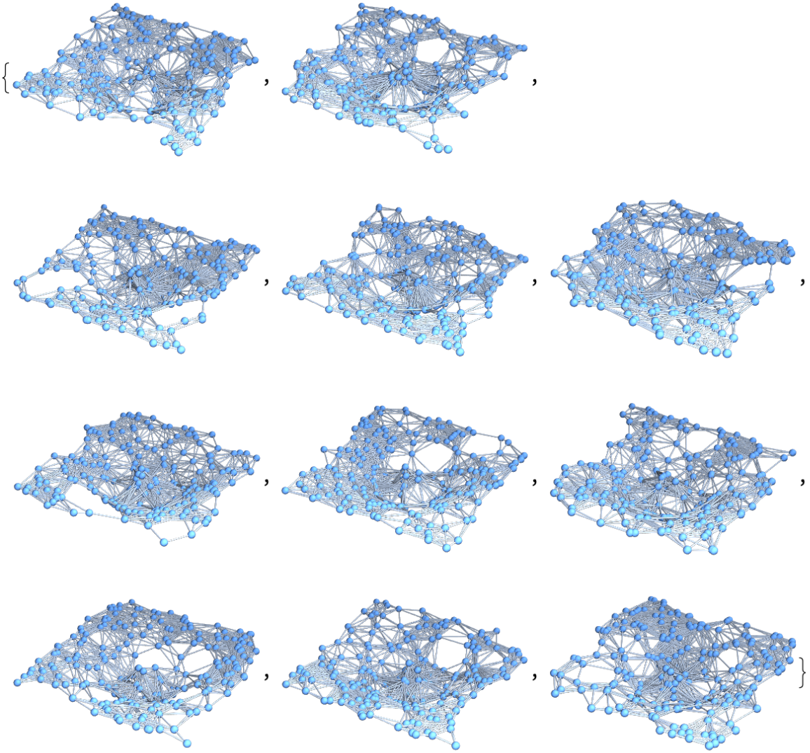 |
Show a list of 3 hypersurfaces (plus initial data) representing the complete "evolution" of the decomposition in Cartesian coordinates, with spatial coordinates based on hypersurface embedding information:
| In[58]:= |
| Out[58]= | 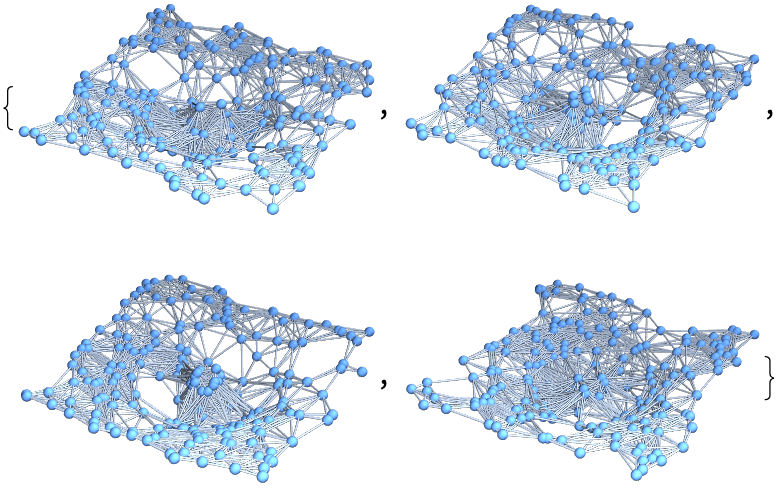 |
Show a list of 10 hypersurfaces (plus initial data) representing the complete "evolution" of the decomposition in Cartesian coordinates:
| In[59]:= |
Show a list of 3 hypersurfaces (plus initial data) representing the complete "evolution" of the decomposition in Cartesian coordinates:
| In[60]:= |
Show the metric tensor for the underlying manifold represented by the discrete hypersurface decomposition:
| In[61]:= |
| Out[61]= |  |
Show the list of coordinate symbols for the discrete hypersurface decomposition:
| In[62]:= |
| Out[62]= |
Show the list of differential 1-form symbols for the coordinates of the discrete hypersurface decomposition:
| In[63]:= |
| Out[63]= |
Show the distinguished "time" coordinate symbol for the discrete hypersurface decomposition:
| In[64]:= |
| Out[64]= |
Show the 1-dimensional interval (range) of the distinguished "time" coordinate for the discrete hypersurface decomposition:
| In[65]:= |
| Out[65]= |
Show the distinguished "spatial" coordinate symbols for the discrete hypersurface decomposition:
| In[66]:= |
| Out[66]= |
Show the 2-dimensional region (range) of the distinguished "spatial" coordinates for the discrete hypersurface decomposition:
| In[67]:= |
| Out[67]= |
Show the number of points (vertices) within each hypersurface of the decomposition:
| In[68]:= |
| Out[68]= |
Show the discretization scale for each hypersurface of the decomposition:
| In[69]:= |
| Out[69]= |
Show the number of dimensions of the underlying manifold represented by the discrete hypersurface decomposition:
| In[70]:= |
| Out[70]= |
Show the signature of the underlying manifold represented by the discrete hypersurface decomposition (with +1s representing positive eigenvalues and -1s representing negative eigenvalues of the metric tensor):
| In[71]:= |
| Out[71]= |
Determine whether the underlying manifold represented by the discrete hypersurface decomposition is Riemannian (i.e. all eigenvalues of the metric tensor have the same sign):
| In[72]:= |
| Out[72]= |
Determine whether the underlying manifold represented by the discrete hypersurface decomposition is pseudo-Riemannian (i.e. all eigenvalues are non-zero, but not all have the same sign):
| In[73]:= |
| Out[73]= |
Determine whether the underlying manifold represented by the discrete hypersurface decomposition is Lorentzian (i.e. all eigenvalues of the metric tensor have the same sign, except for one eigenvalues which has the opposite sign):
| In[74]:= |
| Out[74]= |
Show the list of conditions on the coordinates required to guarantee that the underlying manifold represented by the discrete hypersurface decomposition is Riemannian (i.e. all eigenvalues of the metric tensor are positive):
| In[75]:= |
| Out[75]= |
Show the list of conditions on the coordinates required to guarantee that the underlying manifold represented by the discrete hypersurface decomposition is pseudo-Riemannian (i.e. all eigenvalues of the metric tensor are non-zero):
| In[76]:= |
| Out[76]= |
Show the list of conditions on the coordinates required to guarantee that the underlying manifold represented by the discrete hypersurface decomposition is Lorentzian (i.e. the "time" eigenvalue is negative, and all other eigenvalues are positive):
| In[77]:= |
| Out[77]= |
This work is licensed under a Creative Commons Attribution 4.0 International License