Wolfram Function Repository
Instant-use add-on functions for the Wolfram Language
Function Repository Resource:
Generate a Morton (z-order) curve
ResourceFunction["MortonCurve"][n] gives the line segments representing the nth-step Morton (z-order) curve. | |
ResourceFunction["MortonCurve"][n,d] gives the nth-step Morton curve in d dimensions. |
A 2D z-order curve:
| In[1]:= |
| Out[1]= |  |
Lengths of the approximations to the Morton curve:
| In[2]:= |
| Out[2]= |
Visualize the Morton curve in 2D with splines:
| In[3]:= |
| Out[3]= |  |
A 2D Morton curve:
| In[4]:= |
| Out[4]= |  |
A 3D Morton curve:
| In[5]:= |
| Out[5]= | 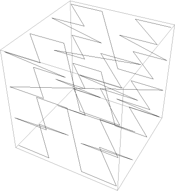 |
An n-dimensional Morton curve:
| In[6]:= |
| Out[6]= |
Show the Morton curve for different numbers of steps:
| In[7]:= |
| Out[7]= |  |
DataRange allows you to specify the range of mesh coordinates to generate:
| In[8]:= |
| Out[8]= |
Specify a different range:
| In[9]:= |
| Out[9]= |  |
Visualize the Morton curve in 3D:
| In[10]:= |
| Out[10]= | 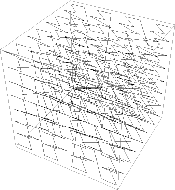 |
With tubes:
| In[11]:= |
| Out[11]= | 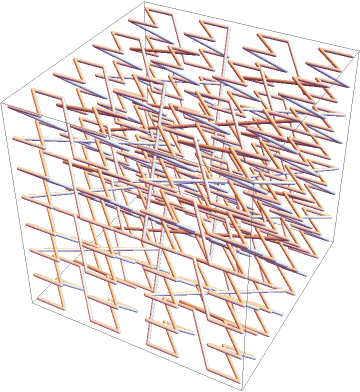 |
MortonCurve consists of lines:
| In[12]:= |
| Out[12]= |
DataRange→range is equivalent to using RescalingTransform[{…},range]:
| In[13]:= |
| Out[13]= | 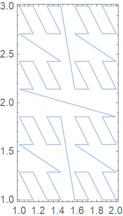 |
Use RescalingTransform directly:
| In[14]:= | ![box = TransformedRegion[ResourceFunction["MortonCurve"][3], RescalingTransform[{{0, 2^3 - 1}, {0, 2^3 - 1}}, {{1, 2}, {1, 3}}]];
Region[box, Frame -> True]](https://www.wolframcloud.com/obj/resourcesystem/images/49e/49e1f79b-7c97-4184-b6a4-082e5ca2ed70/71a8cb13c182c4f5.png) |
| Out[14]= | 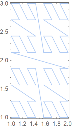 |
By default, the coordinates of the Morton curve are not in the unit square:
| In[15]:= |
| Out[15]= |
Use DataRange to generate the Morton curve in the unit square:
| In[16]:= |
| Out[16]= |  |
MortonCurve can be too large to generate:
| In[17]:= |
| Out[17]= |
Traverse a Morton curve dynamically:
| In[18]:= | ![With[{curve = ResourceFunction["MortonCurve"][6]},
Manipulate[
Graphics[{curve, Red, Thick, Line[Take[First[curve], i]]}, ImageSize -> Medium], {i, 1, 4096, 1}, SaveDefinitions -> True]]](https://www.wolframcloud.com/obj/resourcesystem/images/49e/49e1f79b-7c97-4184-b6a4-082e5ca2ed70/16cdfcc6817bd4f3.png) |
| Out[18]= | 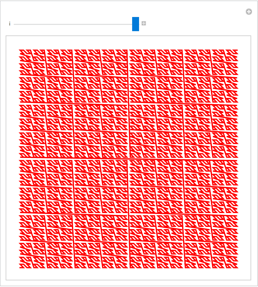 |
This work is licensed under a Creative Commons Attribution 4.0 International License