Details
ResourceFunction["TopolyFunction"] is a wrapper for the Python package
Topoly. The package is installed automatically, as neccessary, using the the resource function
PythonEvaluateWithDependencies.
ResourceFunction["TopolyFunction"] distinguishes knots, slipknots, links and spatial graphs through the calculation of topological polynomial invariants of a structure; identifies lasso types; creates minimal spanning surfaces; and generates random closed polymers.
The Python package Topoly and therefore ResourceFunction["TopolyFunction"] are not supported in Windows.
In ResourceFunction["TopolyFunction"][{"func",structure,…}] and ResourceFunction["TopolyFunction"][{"func",chain,…}], structure or chain can refer to a local or remote file or a Wolfram Language expression.
Files can be specified using a string giving a relative or absolute path to a local file, a
File object or a
URL object.
Accepted file formats include:
| "XYZ" | coordinates in the three or four-column format (with index) |
| "PDB" | protein structure |
| "CIF" | crystallographic structure |
| "WL", "MATH" | coordinates in the Wolfram Language format |
Accepted forms of expressions include:
| {{x1,y1,z1},…} | list of coordinates |
| "pdcode" | planar diagram code string |
| "emcode" | Ewing–Millett code string |
Planar diagram (PD) code and Ewing–Millett (EM) codes are explained in the
PD code and EM code section of the Topoly Dictionary.
Structures can be modified using the following functions:
| "StructureClose" | connects loose ends |
| "StructureReduce" | reduces the number of crossings |
Functions that are capable of automatically performing structure modifications accept the options "Closure" and "ReductionMethod" with the same option values as "StructureClose" and "StructureReduce", respectively.
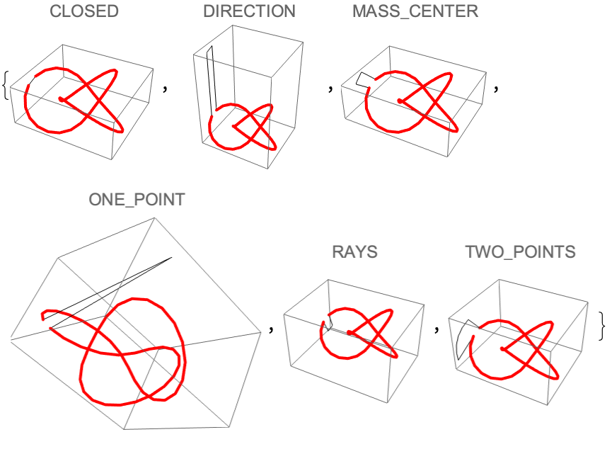
The method for connecting loose ends is chosen using the "Closure" option, which involves either a straight line or a path along an encompassing sphere with the center at the geometric center of the structure. The available methods include:
| "CLOSED" | straight line |
| "MASS_CENTER" | endpoints projections in the direction from the center of mass |
| "DIRECTION" | parallel segments from the endpoints in a chosen direction |
| "ONE_POINT" | the endpoints connected to a single randomly chosen point |
| "TWO_POINTS" | two random points (default) |
| "RAYS" | parallel segments from the endpoints in a random direction |
The structure reduction method is chosen usign the option "ReductionMethod" with the following possible values:
ResourceFunction["TopolyFunction"]["Properties"] gives a list of the available function properties.
Functions for calculating topological invariants include:
| "AlexanderPolynomial" | Alexander polynomial |
| "APSBracket" | APS bracket |
| "BLMHoPolynomial" | BLM/Ho polynomial |
| "ConwayPolynomial" | Conway polynomial |
| "HOMFLYPolynomial" | HOMFLY polynomial |
| "JonesPolynomial" | Jones polynomial |
| "KauffmanBracket" | Kauffman bracket |
| "KauffmanPolynomial" | Kauffman two-variable polynomial |
| "Writhe" | writhe |
| "YamadaPolynomial" | Yamada polynomial |
With the default value of the option
"Matrix"→False, invariant functions generally return the topology type for deterministic values of the option "Closure" and an association of topology types and their probabilities for randomized values of
"Closure". For
"Matrix"→True, these values are returned in an association with subchain indices as keys.
When detected, the polynomial notations for topology type strings returned by the Python code are converted to Wolfram Language expressions as follows:
| "n_k" | Alexander–Briggs notation nk |
| "i1 i2 i3…" | polynomial coefficient lists {i1,i2,i3,…} |
| "polynomial" | polynomial as a pure function |
Functions for analyzing subchain topology include:
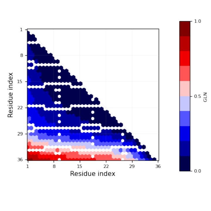
| "GaussLinkingNumber" | Gauss linking number (GLN) between two chains |
| "FindSpots" | centers of fields in the knotting fingerprint matrix |
| "MatrixConvert" | converts between fingeprint matrix formats |
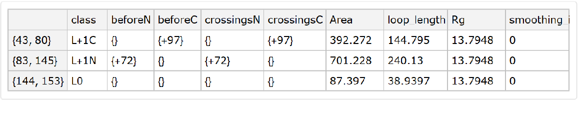
Functions for the lasso type identification include:
| "LassoType" | lasso types for loops |
| "MinimalSurfaceMesh" | triangulated minimal surface spanning a loop |
Functions for finding loops, links, theta-curves and handcuffs include:
| "FindLoops" | loops |
| "FindLinks" | links |
| "FindThetas" | theta-curves |
| "FindHandcuffs" | handcuffs |
Functions for converting between different structure representations include:
| {"TopologyTypeToPDCode","type"} | topology type to PD code |
| {"StructureConvert","code"} | PD code to EM code and vice versa |
| {"CoefficientsToTopologyType",coef,"invariant"} | polynomial coefficients to topology type |
Coefficients coef can be given as:
| {c1,c2,…} | list |
| "c1 c2 …" | string of space-delimited coefficients |
| <|coef1→prob1,…|> | association of coefficients and their probabilities |
Possible specifications for "invariant" include:
| "Alexander" | Alexander polynomial |
| "Jones" | Jones polynomial |
| "Conway" | Conway polynomial |
| "HOMFLY" | HOMFLY polynomial |
| "Yamada" | Yamada polynomial |
| "APS" | APS bracket |
Functions that generate coordinates of n random polygons include:
| {"RandomWalk",k,n} | k-step random walks |
| {"RandomLoop",k,n} | length k loops |
| {"RandomLasso",k,l,n} | lassos with loop length of k and tail length of l |
| {"RandomHandcuff",{k,l},m,n} | handcuffs with loops of length k and l and tail length of m |
| {"RandomLink",{k,l},d,n} | loop pairs of length k and l and distance between their geometric centers of d |
In ResourceFunction["TopolyFunction"]["Information",comp,…], comp can be a function name or a parameter class. Possible elements of the returned association include:
| "Arguments" | arguments of the function |
| "Options" | options of the function |
| "Values" | possible values of the component |
ResourceFunction["TopolyFunction"]["PropertyRules"] provides a mapping between the property names and the underlying Python-side names.
ResourceFunction["TopolyFunction"]["RawInformation",func,…] returns a string representing the Python-side help for the function func.
In ResourceFunction["TopolyFunction"], strings representing function names, option names and option values can be given as either property names or Python-side names.


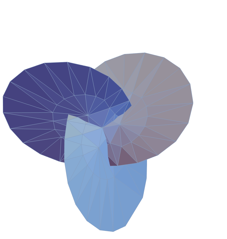
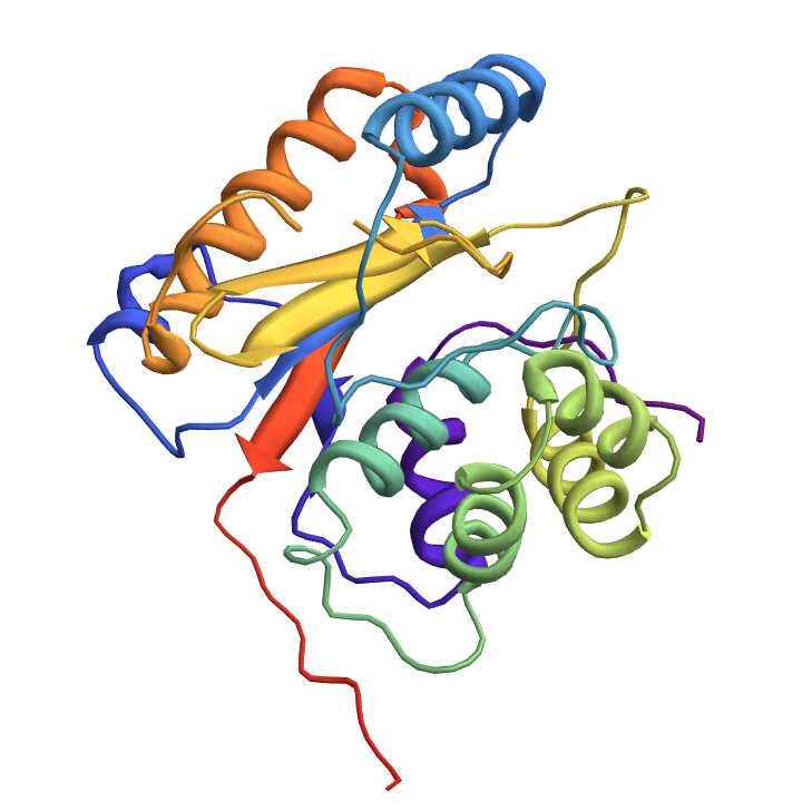
![mesh = ResourceFunction[
"TopolyFunction"][{"MinimalSurfaceMesh", coordinates, "LoopIndices" -> {1, Length[coordinates]}}]](https://www.wolframcloud.com/obj/resourcesystem/images/477/477ac74e-dcfd-44c6-b18e-35d111a2e3be/374378b2061bddab.png)

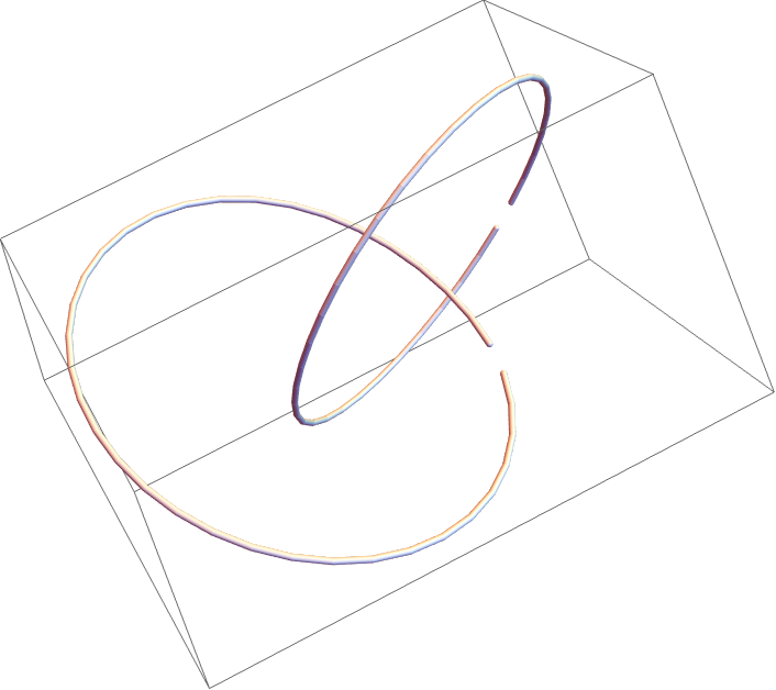
![ResourceFunction[
"TopolyFunction"][{"AlexanderPolynomial", URL["https://people.math.sc.edu/Burkardt/data/xyz/helix_201.xyz"], "Closure" -> "CLOSED"}]](https://www.wolframcloud.com/obj/resourcesystem/images/477/477ac74e-dcfd-44c6-b18e-35d111a2e3be/23183ece5a074ddf.png)
![ResourceFunction[
"TopolyFunction"][{"AlexanderPolynomial", URL["https://raw.githubusercontent.com/ilbsm/topoly_tutorial/master/data/1j85.math"], "Closure" -> "CLOSED"}]](https://www.wolframcloud.com/obj/resourcesystem/images/477/477ac74e-dcfd-44c6-b18e-35d111a2e3be/2f4768cc9308be68.png)
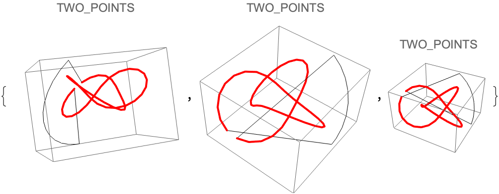
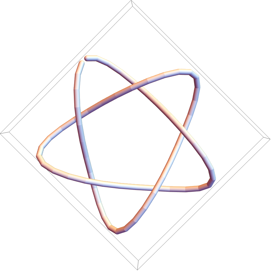
![Table[Graphics3D[{Line[
joinEnds@ ResourceFunction[
"TopolyFunction"][{"StructureClose", coordinates, "Closure" -> closure}]], {Thick, Red, Line[coordinates]}}, PlotLabel -> closure], {closure, ResourceFunction["TopolyFunction"]["Information", "Closure"][
"Values"]}]](https://www.wolframcloud.com/obj/resourcesystem/images/477/477ac74e-dcfd-44c6-b18e-35d111a2e3be/275fa0aef57cc853.png)
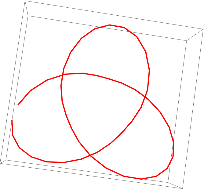
![Table[Graphics3D[{Line[
joinEnds@ ResourceFunction[
"TopolyFunction"][{"StructureClose", coordinates, "Closure" -> closure}]], {Thick, Red, Line[coordinates]}}, PlotLabel -> closure], {3}]](https://www.wolframcloud.com/obj/resourcesystem/images/477/477ac74e-dcfd-44c6-b18e-35d111a2e3be/5c0b9b1ebef46b4a.png)


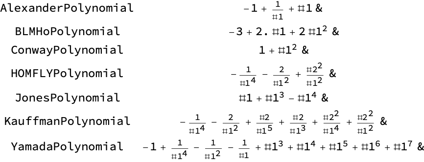
![Table[{poly, ResourceFunction[
"TopolyFunction"][{poly, coordinates, "ReducedPolynomials" -> False, "Translate" -> False, "Closure" -> "CLOSED"}]}, {poly, Select[ ResourceFunction["TopolyFunction"]["Properties"], StringContainsQ[#, "Polynomial"] &]}] // Grid](https://www.wolframcloud.com/obj/resourcesystem/images/477/477ac74e-dcfd-44c6-b18e-35d111a2e3be/07e9f95502aac47b.png)
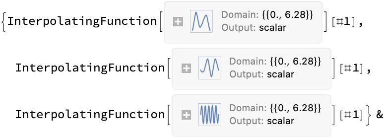
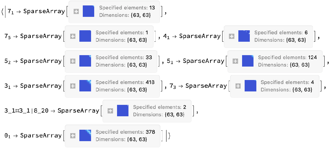
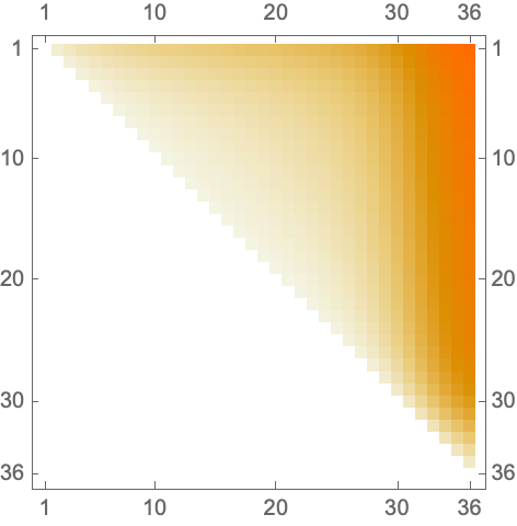
![PrintTemporary["This may take a while..."];
(assoc = ResourceFunction[
"TopolyFunction"][{"ConwayPolynomial", coordinates51, "Tries" -> 10, "Matrix" -> True, "MatrixMap" -> True, "MapFilename" -> filename}]) // Short](https://www.wolframcloud.com/obj/resourcesystem/images/477/477ac74e-dcfd-44c6-b18e-35d111a2e3be/04eca42f57db4c6d.png)

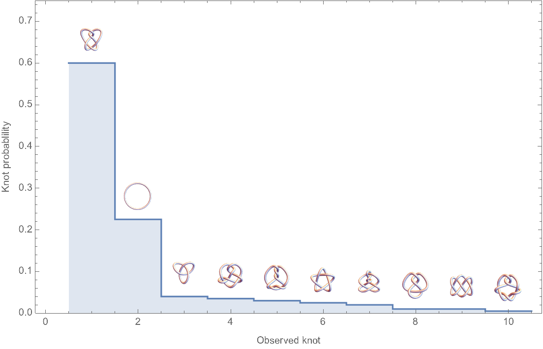
![Module[{keys = Keys[stats], iconF},
iconF[sub_Subscript] := KnotData[List @@ sub];
iconF[_] := ""; ListStepPlot[KeyValueMap[Labeled[#2, iconF[#], Top] &, stats], Center, Ticks -> {Transpose[{Range[Length[keys]], keys}], Automatic}, PlotRangePadding -> {Automatic, {0, 0.15}}, Filling -> Bottom, Frame -> True, FrameLabel -> {"Observed knot", "Knot probablility"}]]](https://www.wolframcloud.com/obj/resourcesystem/images/477/477ac74e-dcfd-44c6-b18e-35d111a2e3be/2bf812daa3a5013d.png)
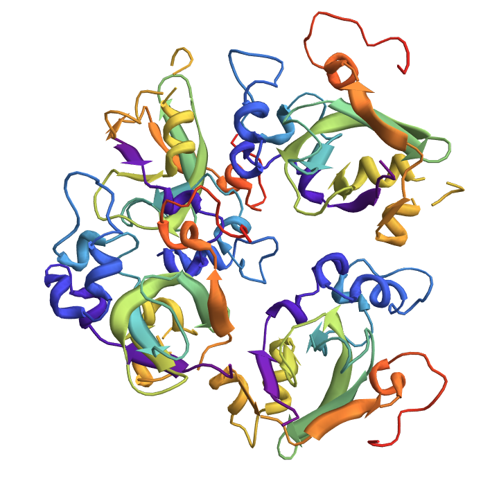

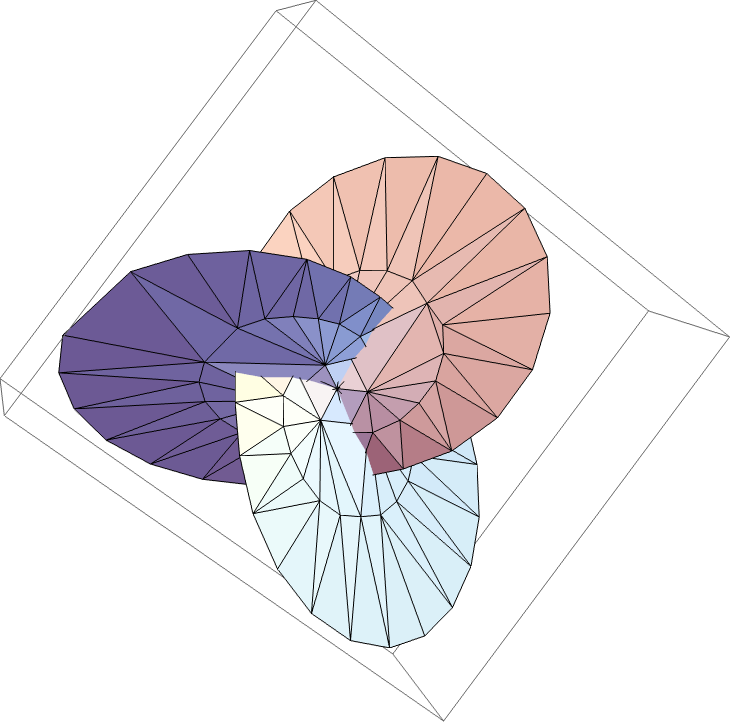
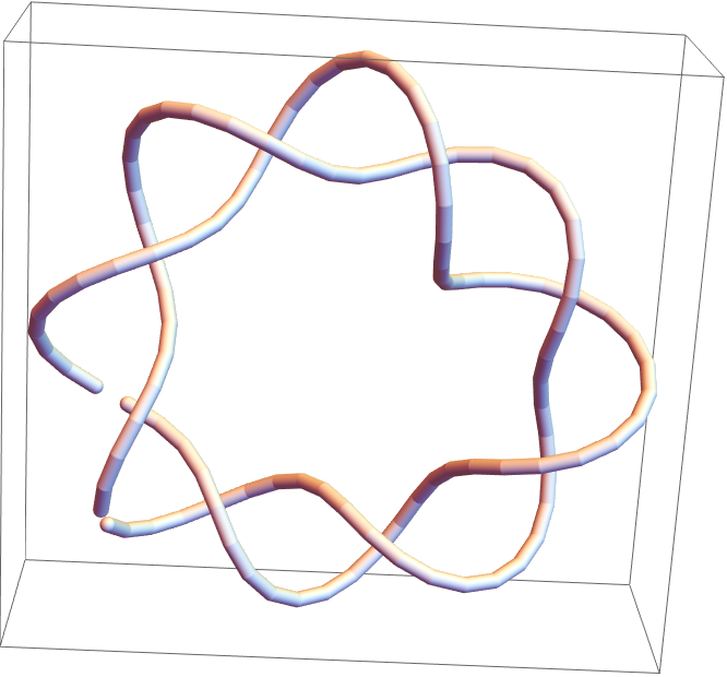
![meshes = KeyValueMap[
Show[ ResourceFunction[
"TopolyFunction"][{"MinimalSurfaceMesh", file, "LoopIndices" -> #}], PlotLabel -> #2["class"]] &, lassos]](https://www.wolframcloud.com/obj/resourcesystem/images/477/477ac74e-dcfd-44c6-b18e-35d111a2e3be/2c561450448502df.png)