Wolfram Function Repository
Instant-use add-on functions for the Wolfram Language
Function Repository Resource:
Smooth noisy data using local regression
ResourceFunction["Loess"][data, bandwidth, x] finds the interpolation of data at x by using local regression smoothing of bandwidth data points. | |
ResourceFunction["Loess"][data, Scaled[bandwidth], x] finds the interpolation of data at x by using local regression smoothing of bandwidth fraction of data points. | |
ResourceFunction["Loess"][data,bandwidth,{x1,x2,…}] finds the interpolation of data at each xi by using local regression smoothing of bandwidth data points. |
Loess is useful when data is noisy but has an underlying trend:
| In[1]:= |
| Out[2]= | 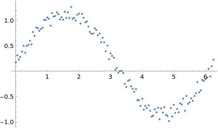 |
Find an estimated value for the data at x=2 using the nearest 12 data points:
| In[3]:= |
| Out[3]= |
Find an estimated value for the data at x=2 using the nearest 10% of the data:
| In[4]:= |
| Out[4]= |
| In[5]:= |
| Out[5]= | 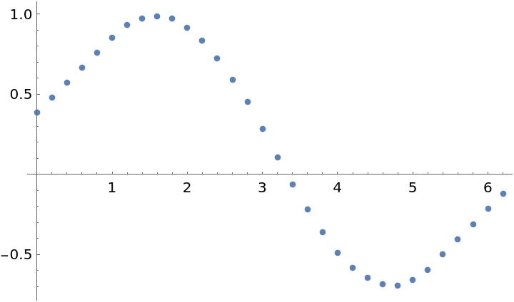 |
Loess can handle higher-dimensional data:
| In[6]:= |
| Out[7]= | 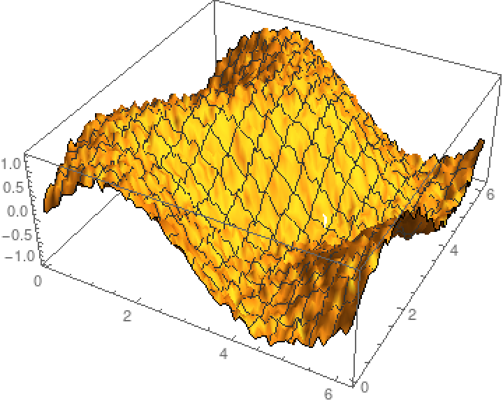 |
| In[8]:= |
| Out[8]= |
| In[9]:= |
| Out[9]= | 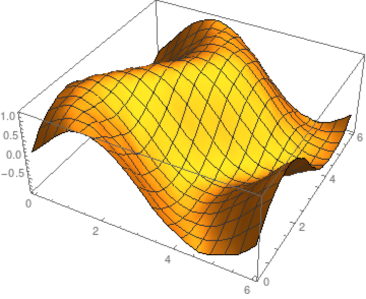 |
By default, Loess fits straight lines to subsets of data, but you can increase the interpolation order to capture different detail:
| In[10]:= |
| Out[11]= | 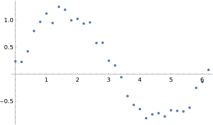 |
| In[12]:= |
| Out[12]= | 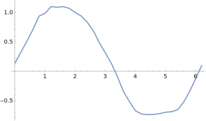 |
| In[13]:= |
| Out[13]= | 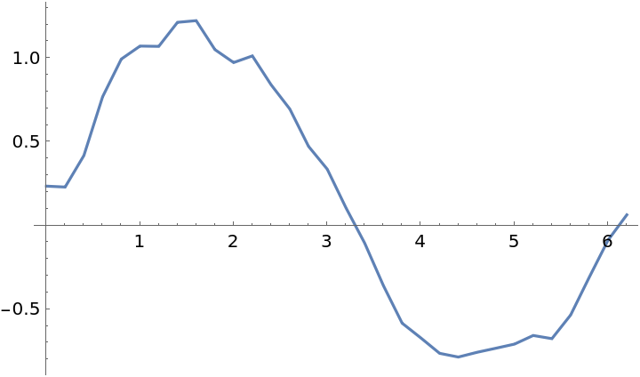 |
Loess fitting involves weighting the local data. Typically, points further from the estimated point are given less weight:
| In[14]:= | ![ListLinePlot[
Table[{x, ResourceFunction["Loess"][data, Scaled[0.2], x, "WeightsFunction" -> (1/(0.1 + Norm[#]) &)]}, {x, 0, 2 \[Pi], 0.2}]]](https://www.wolframcloud.com/obj/resourcesystem/images/471/471a48a8-b284-46b3-9034-e238ac8d9464/04c57a36d6d6c23c.png) |
| Out[14]= | 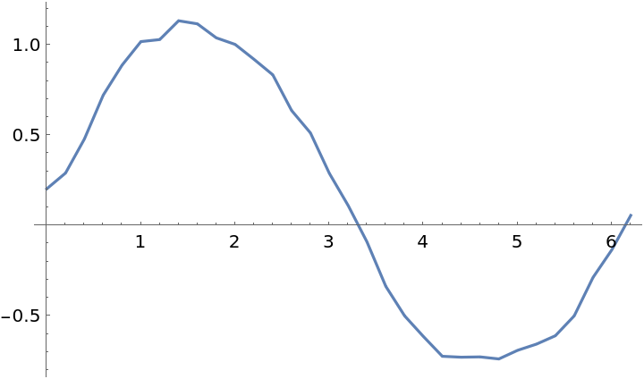 |
If you intend to use Loess to predict many values from the same data, then it is more efficient to find all values in a single request:
| In[15]:= |
| Out[16]= | 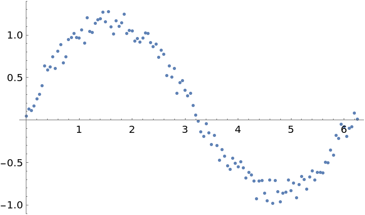 |
This method:
| In[17]:= | ![xvals = Range[0, 2 \[Pi], 0.2];
ListPlot[
Transpose[{xvals, ResourceFunction["Loess"][data, 40, xvals]}]]](https://www.wolframcloud.com/obj/resourcesystem/images/471/471a48a8-b284-46b3-9034-e238ac8d9464/1ff90f912a43e5a0.png) |
| Out[13]= |  |
Is faster than this method:
| In[18]:= |
| Out[18]= | 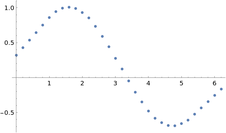 |
Wolfram Language 11.3 (March 2018) or above
This work is licensed under a Creative Commons Attribution 4.0 International License