Wolfram Function Repository
Instant-use add-on functions for the Wolfram Language
Function Repository Resource:
Get curves defined over a sphere
ResourceFunction["SphericalCurve"][{par1,par2,…},"type"] gives the parametrization of a curve of the given type on a sphere, with parameters pari. |
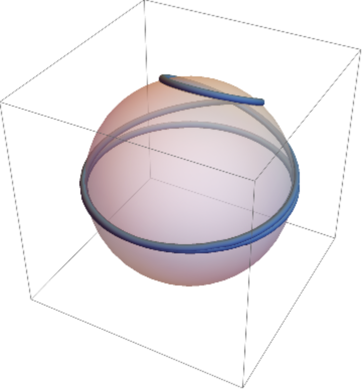
Get the expression for a hyperbolic tangent spiral on a sphere:
| In[1]:= |
|
| Out[1]= |
|
Plot it:
| In[2]:= |
![Show[ParametricPlot3D[Evaluate[hts],
{t, -10, 10}, Axes -> None, PlotStyle -> Tube[.035]], Graphics3D[{Opacity[.5], Sphere[{0, 0, 0}, .99]}], PlotRange -> All]](https://www.wolframcloud.com/obj/resourcesystem/images/461/461d3ea4-e527-45fd-9be5-b918be50c3f6/5fdb622ba4f67a76.png)
|
| Out[2]= |
|
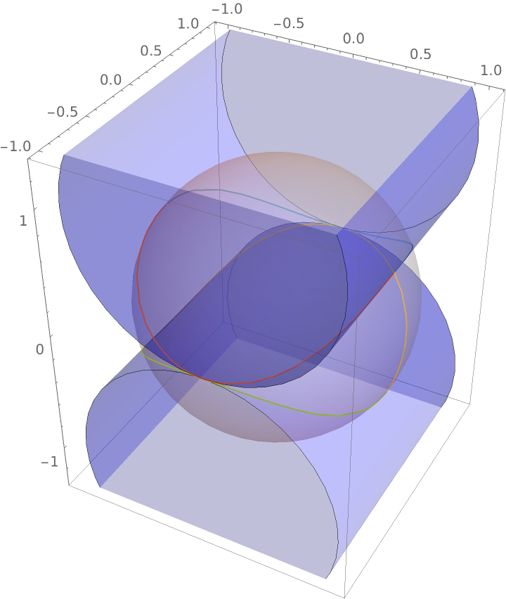
A sphero-cylindrical curve is the intersections between a sphere and a cylinder of revolution:
| In[3]:= |
![Show[ParametricPlot3D[
Evaluate[{ResourceFunction["SphericalCurve"][{1, -1, 1}, t, "SpheroCylindricalCurve"], ResourceFunction["SphericalCurve"][{1, -1, -1}, t, "SpheroCylindricalCurves"], -ResourceFunction[
"SphericalCurve"][{1, -1, 1}, t, "SpheroCylindricalCurves"], -ResourceFunction[
"SphericalCurve"][{1, -1, -1}, t, "SpheroCylindricalCurves"]}], {t, -\[Pi], \[Pi]}, Axes -> True],
Graphics3D[{Opacity[.25], Sphere[{0, 0, 0}, 1], Blue, Cylinder[{{0, 1, 1}, {0, -1., 1}}], Cylinder[{{0, 1, -1}, {0, -1., -1}}]}]]](https://www.wolframcloud.com/obj/resourcesystem/images/461/461d3ea4-e527-45fd-9be5-b918be50c3f6/538120798221a3f0.png)
|
| Out[3]= |
|
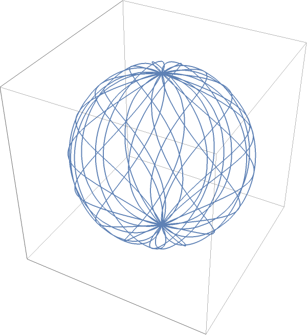
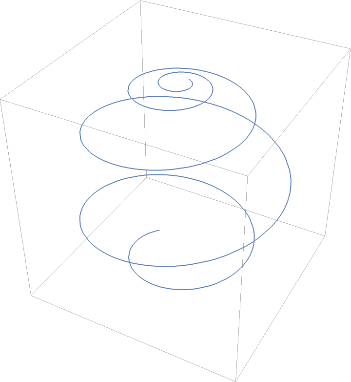
Seiffert's spherical spiral:
| In[4]:= |
![ParametricPlot3D[
ResourceFunction["SphericalCurve"][{1, .5}, t, "SeiffertsSphericalSpiral"], {t, 0, 100}, Ticks -> None]](https://www.wolframcloud.com/obj/resourcesystem/images/461/461d3ea4-e527-45fd-9be5-b918be50c3f6/22d0684906e4c767.png)
|
| Out[4]= |
|
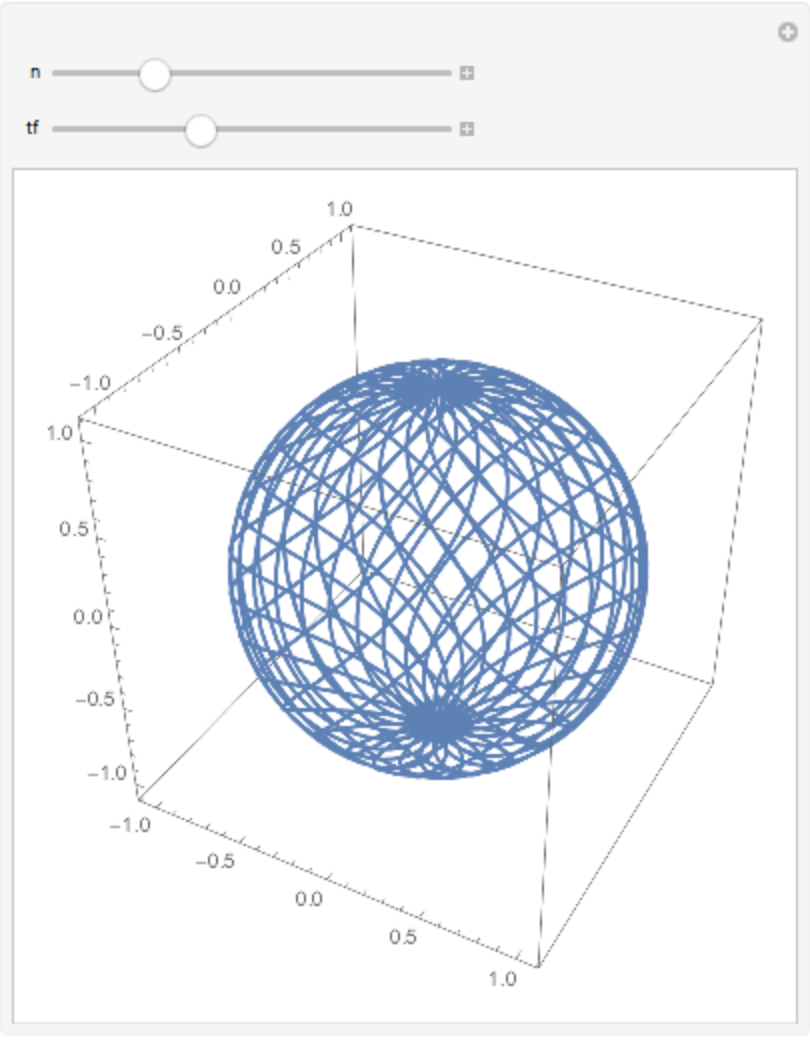
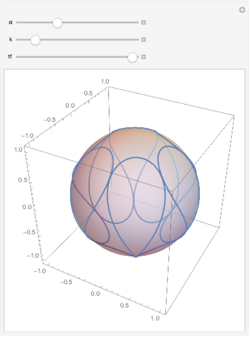
The Clelia:
| In[5]:= |
![Manipulate[
ParametricPlot3D[
Evaluate[ResourceFunction["SphericalCurve"][{1, n}, t, "Clelia"]], {t, 0, tf}, Axes -> True, PlotRange -> All], {{n, 115/100}, 0, 5}, {{tf, 180}, 1, 500}]](https://www.wolframcloud.com/obj/resourcesystem/images/461/461d3ea4-e527-45fd-9be5-b918be50c3f6/24ff352e0dc205ea.png)
|
| Out[5]= |
|
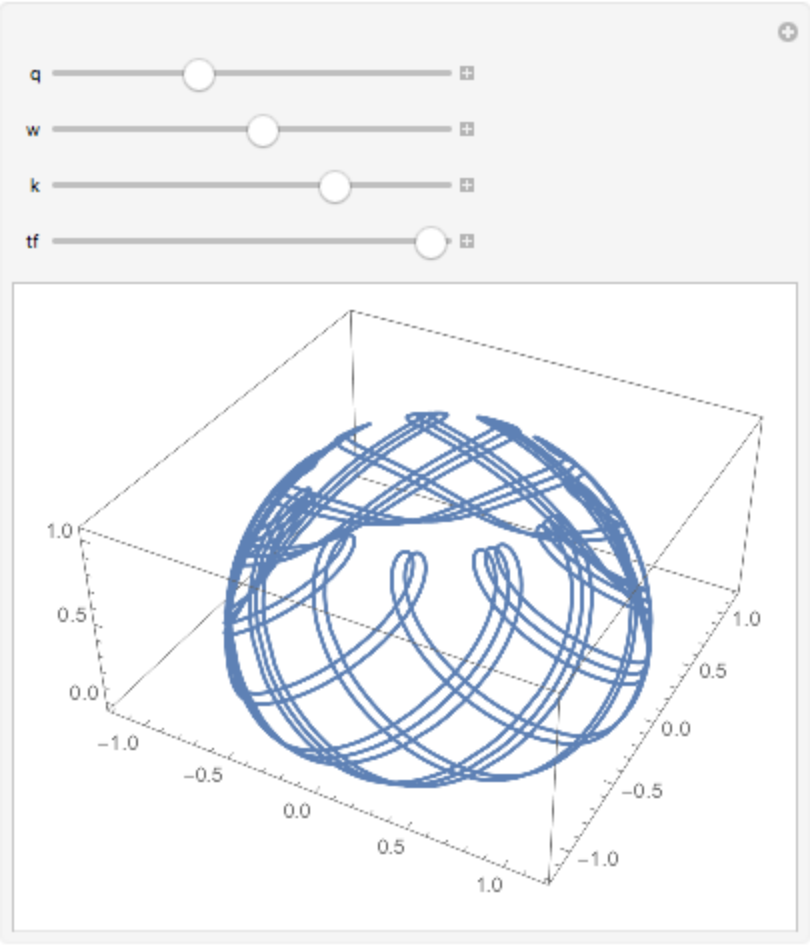
Spherical cycloid:
| In[6]:= |
![Manipulate[
ParametricPlot3D[
Evaluate[ResourceFunction["SphericalCurve"][{1, q, w, k}, t, "SphericalCycloid"]], {t, 0, tf}, Axes -> True, PlotRange -> All], {{q, 1.1}, 0, \[Pi]}, {{w, .532}, 0, 1}, {{k, .734}, 0, 1}, {{tf, 250}, 1, 250}]](https://www.wolframcloud.com/obj/resourcesystem/images/461/461d3ea4-e527-45fd-9be5-b918be50c3f6/052c22964587c8a0.png)
|
| Out[6]= |
|
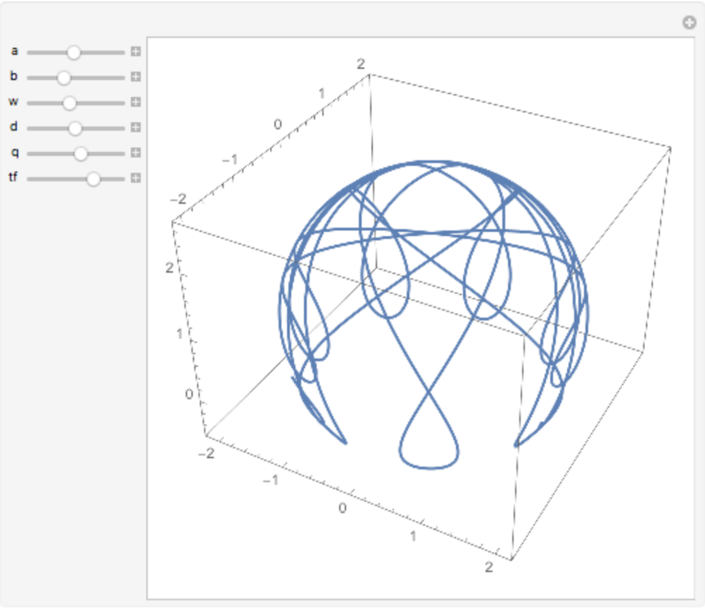
Spherical trochoid:
| In[7]:= |
![Manipulate[ParametricPlot3D[
Evaluate[
ResourceFunction["SphericalCurve"][{a, b, w, d, q}, t, "SphericalTrochoid"]], {t, 0, tf},
Axes -> True, PlotRange -> All], {{a, 1.5}, 0, \[Pi], ImageSize -> Tiny}, {{b, 1.1}, 0, \[Pi], ImageSize -> Tiny}, {{w, 1.31}, 0, \[Pi], ImageSize -> Tiny}, {{d, 1.55}, 0, \[Pi], ImageSize -> Tiny}, {{q, 1.77}, 0, \[Pi], ImageSize -> Tiny}, {{tf, 36}, 1, 50, ImageSize -> Tiny}, ControlPlacement -> Left]](https://www.wolframcloud.com/obj/resourcesystem/images/461/461d3ea4-e527-45fd-9be5-b918be50c3f6/25bb635bddce6f20.png)
|
| Out[7]= |
|
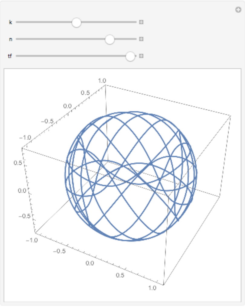
Spherical sinusoid:
| In[8]:= |
![Manipulate[
ParametricPlot3D[
Evaluate[ResourceFunction["SphericalCurve"][{1, k, n}, t, "SphericalSinusoid"]], {t, 0, tf}, Axes -> True, PlotRange -> All], {{k, 1}, 0, 2}, {{n, 1.625}, 0, 2}, {{tf, 150}, 0, 150}]](https://www.wolframcloud.com/obj/resourcesystem/images/461/461d3ea4-e527-45fd-9be5-b918be50c3f6/3a0e255e577b4067.png)
|
| Out[8]= |
|
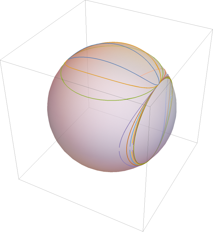
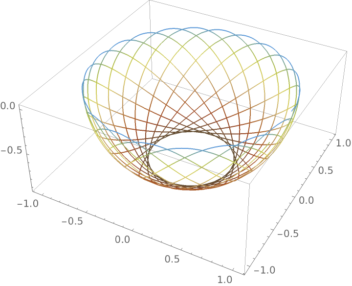
Spherical ellipses:
| In[9]:= |
![Show[ParametricPlot3D[
Evaluate[Table[
ResourceFunction["SphericalCurve"][{4, 3, c, 1}, t, "SphericalEllipse"], {c, 1, 10, 1}]], {t, 0, 4 \[Pi]}, Axes -> None], Graphics3D[{Opacity[.5], Sphere[{0, 0, 0}, 3.99]}], PlotRange -> All]](https://www.wolframcloud.com/obj/resourcesystem/images/461/461d3ea4-e527-45fd-9be5-b918be50c3f6/5076b0bec06456b2.png)
|
| Out[9]= |
|
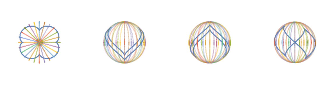
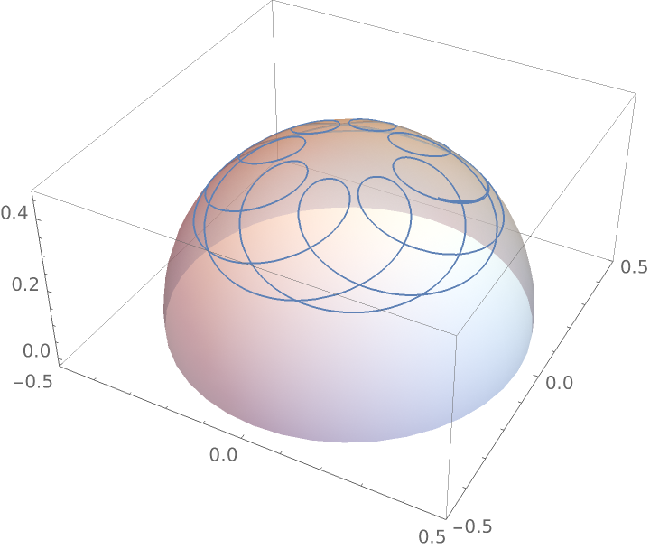
Spherical helix:
| In[10]:= |
![meridians[gl_] := ParametricPlot3D[
Evaluate[Table[
1 {Cos[u] Cos[v], Sin[u] Cos[v], Sin[v]}, {u, 0, 2 \[Pi], gl}]], {v, -(\[Pi]/2), \[Pi]/2}, PlotStyle -> Opacity[.25]]](https://www.wolframcloud.com/obj/resourcesystem/images/461/461d3ea4-e527-45fd-9be5-b918be50c3f6/36731dd4ce9eaad4.png)
|
| In[11]:= |
![With[{m = meridians[2 \[Pi]/24]},
GraphicsRow[
Show[ParametricPlot3D[
Evaluate[
ResourceFunction["SphericalCurve"][{2/3, 1/6}, t, "SphericalHelix"]], {t, 0, 2 \[Pi]}, Axes -> None, Boxed -> False, ViewPoint -> #], m] & /@ {Above, Front, Left, {Left, Front}}, ImageSize -> Full]]](https://www.wolframcloud.com/obj/resourcesystem/images/461/461d3ea4-e527-45fd-9be5-b918be50c3f6/1389d57bcf60ad4d.png)
|
| Out[11]= |
|
Spherical cardioid:
| In[12]:= |
![Show[ParametricPlot3D[
Evaluate[ResourceFunction["SphericalCurve"][{1}, t, "SphericalCardioid"]],
{t, 0, 4 \[Pi]}, Axes -> None], Graphics3D[{Opacity[.5], Sphere[{0, 0, 0}, 2.99]}]]](https://www.wolframcloud.com/obj/resourcesystem/images/461/461d3ea4-e527-45fd-9be5-b918be50c3f6/1ed52901caa4ca36.png)
|
| Out[12]= |
|
Satellite curve (Clelias and the spherical helices are special cases):
| In[13]:= |
![Manipulate[
Show[ParametricPlot3D[
Evaluate[
ResourceFunction["SphericalCurve"][{1, k, \[Alpha]}, t, "SatelliteCurve"]], {t, 0, tf}, Axes -> True, PlotRange -> All], Graphics3D[{Opacity[.5], Sphere[{0, 0, 0}, .99]}]], {{\[Alpha], 3 \[Pi]/4}, 0, 2 \[Pi]}, {{k, 3}, 0, 10}, {{tf, 4 \[Pi]}, 1, 50}]](https://www.wolframcloud.com/obj/resourcesystem/images/461/461d3ea4-e527-45fd-9be5-b918be50c3f6/02c59999214e5323.png)
|
| Out[13]= |
|
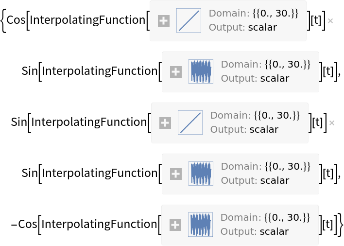
Spherical pendulum:
| In[14]:= |
![sp = ResourceFunction[
"SphericalCurve"][{1(*longitude*), 1(*mass*), 1.57(*initial angle \[Theta]*), 0(*initial velocity \[Theta]*), 0(*initial angle \[CurlyPhi]*), 2(*angular momentum \[CurlyPhi]*)},
30, "SphericalPendulum"]](https://www.wolframcloud.com/obj/resourcesystem/images/461/461d3ea4-e527-45fd-9be5-b918be50c3f6/0c4cdb8c12d1fcda.png)
|
| Out[14]= |
|
Plot the curve:
| In[15]:= |
|
| Out[15]= |
|
Stationary precession of a spinning top:
| In[16]:= |
![Show[ResourceFunction[
"SphericalCurve"][{30(*initial nutation angle*), 10(*g*), 1(*transversal I*), 1(*initial spin*), 1(*longitudinal J*), .25(*height of center of mass*), .5(*mass*), 0.5(*initial nutation velocity*)}, 35, "SpinningTop"], Graphics3D[{Opacity[.5], Sphere[{0, 0, 0}, .45]}]]](https://www.wolframcloud.com/obj/resourcesystem/images/461/461d3ea4-e527-45fd-9be5-b918be50c3f6/06a51f63071456c3.png)
|
| Out[16]= |
|
Spherical rhumb line:
| In[17]:= |
|
| Out[17]= |
|
| In[18]:= |
![ParametricPlot3D[
Evaluate[ResourceFunction["SphericalCurve"][{.15}, t, "SphereRhumbLine"]],
{t, -10, 20}, Axes -> None, BoxRatios -> {1, 1, 1}]](https://www.wolframcloud.com/obj/resourcesystem/images/461/461d3ea4-e527-45fd-9be5-b918be50c3f6/19ac882ae182348c.png)
|
| Out[18]= |
|
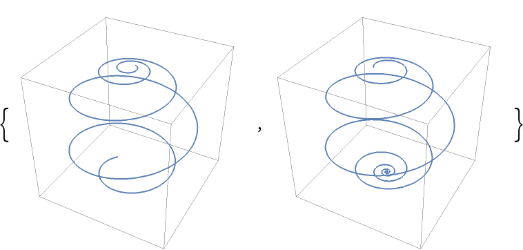
Spherical loxodrome:
| In[19]:= |
|
| Out[19]= |
|
Comparing with the unit–speed spherical loxodrome:
| In[20]:= |
![ParametricPlot3D[
Evaluate[ResourceFunction["SphericalCurve"][{1, 1, .15}, t, #]],
{t, -10, 20}, Axes -> None, BoxRatios -> {1, 1, 1}] & /@ {"SphericalLoxodrome", "SphericalLoxodromeUnitSpeed"}](https://www.wolframcloud.com/obj/resourcesystem/images/461/461d3ea4-e527-45fd-9be5-b918be50c3f6/19313b03b307e24a.png)
|
| Out[20]= |
|
Compute quantities like ArcLength:
| In[21]:= |
|
| Out[21]= |
|
Compute the curvature:
| In[22]:= |
![ResourceFunction["Curvature"][
ResourceFunction["SphericalCurve"][{1}, t, "SphericalCardioid"], t] // FullSimplify](https://www.wolframcloud.com/obj/resourcesystem/images/461/461d3ea4-e527-45fd-9be5-b918be50c3f6/418e72f30fada0e0.png)
|
| Out[22]= |
|
The torsion:
| In[23]:= |
![ResourceFunction["CurveTorsion"][
ResourceFunction["SphericalCurve"][{1}, t, "SphericalCardioid"], t] // FullSimplify](https://www.wolframcloud.com/obj/resourcesystem/images/461/461d3ea4-e527-45fd-9be5-b918be50c3f6/2fe784631559bb63.png)
|
| Out[23]= |
|
The spherical nephroid:
| In[24]:= |
|
The Frenet–Serret system of the curve:
| In[25]:= |
![(* Evaluate this cell to get the example input *) CloudGet["https://www.wolframcloud.com/obj/ba1ea694-b2c2-43fe-a1b8-1e1d56073d9f"]](https://www.wolframcloud.com/obj/resourcesystem/images/461/461d3ea4-e527-45fd-9be5-b918be50c3f6/47ddef26badfe796.png)
|
| Out[25]= |
|
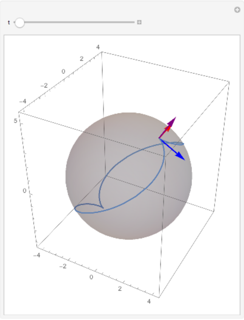
Plot the Frenet–Serret system:
| In[26]:= |
![{tangent, normal, binormal} = Map[Arrow[{sn, sn + 2 #}] &, basis] // PowerExpand // FullSimplify;
plot = ParametricPlot3D[Evaluate[sn], {t, 0, 2 \[Pi]}];
Manipulate[
Evaluate[Show[plot, Graphics3D[{Thick, Blue, tangent, Red, normal, Purple, binormal, Gray, Opacity[0.25], Sphere[{0, 0, 0}, 4]}], PlotRange -> All]], {t, 0, 2 \[Pi]}]](https://www.wolframcloud.com/obj/resourcesystem/images/461/461d3ea4-e527-45fd-9be5-b918be50c3f6/13f7f2c9074eafed.png)
|
| Out[26]= |
|
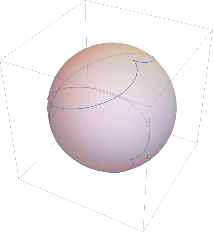
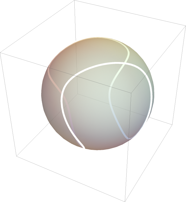
The seam line of a tennis ball:
| In[27]:= |
![Show[ParametricPlot3D[
ResourceFunction["SphericalCurve"][{2, 2, 2, 1}, t, "TennisBallSeam"], {t, 0, 2 \[Pi]}, Axes -> None, PlotPoints -> 150, PlotStyle -> {{White, Thickness[.01]}}], Graphics3D[{Opacity[.5], LightGreen, Sphere[]}]]](https://www.wolframcloud.com/obj/resourcesystem/images/461/461d3ea4-e527-45fd-9be5-b918be50c3f6/3af998fdd8b2ca8b.png)
|
| Out[27]= |
|
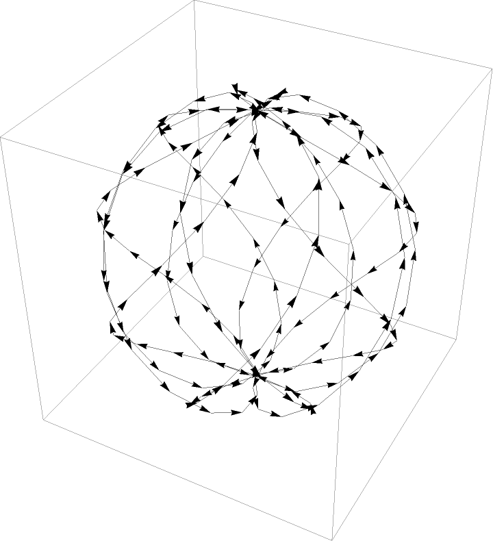
Spherical Lissajous:
| In[28]:= |
![Graphics3D[{Arrowheads[.02], ResourceFunction["ApproximatedCurve"][
ResourceFunction["SphericalCurve"][{3, 5, 7}, t, "SphericalLissajous"], {t, 0, 2 \[Pi], 150}, "Arrow"]}]](https://www.wolframcloud.com/obj/resourcesystem/images/461/461d3ea4-e527-45fd-9be5-b918be50c3f6/54a263cb78587af5.png)
|
| Out[28]= |
|
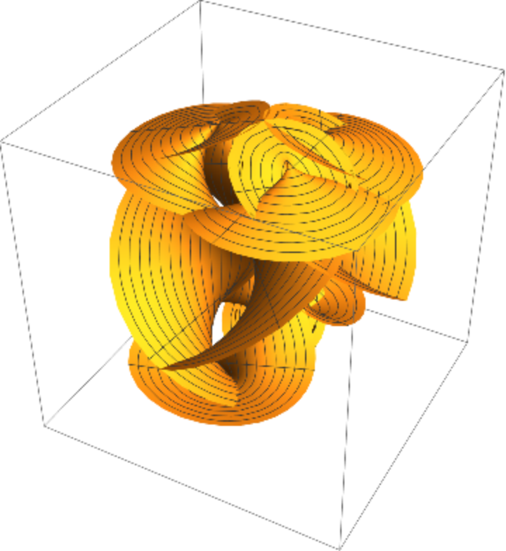
Distinct types of surfaces (like ruled surfaces) can be constructed from curves (used in fields like architecture):
| In[29]:= |
![ParametricPlot3D[
Evaluate[ResourceFunction["NormalSurface"][
ResourceFunction["SphericalCurve"][{3, 7, 5}, t, "SphericalSpiral"], t, {u, v}]],
{u, 0, \[Pi]}, {v, 0, \[Pi]}, PlotPoints -> 60, Axes -> None]](https://www.wolframcloud.com/obj/resourcesystem/images/461/461d3ea4-e527-45fd-9be5-b918be50c3f6/51700343a188cb2b.png)
|
| Out[29]= |
|
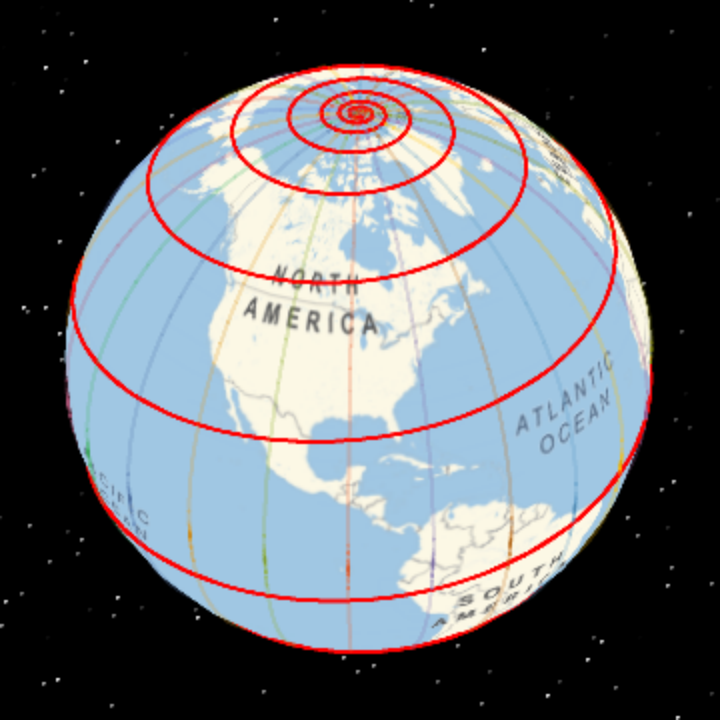
Meridians and loxodrome:
| In[30]:= |
![meridians[gl_] := ParametricPlot3D[
Evaluate[Table[{Cos[u] Cos[v], Sin[u] Cos[v], Sin[v]}, {u, 0, 2 \[Pi], gl}]], {v, -(\[Pi]/2), \[Pi]/2}, PlotStyle -> Opacity[.25]]](https://www.wolframcloud.com/obj/resourcesystem/images/461/461d3ea4-e527-45fd-9be5-b918be50c3f6/27d676b302eb27ad.png)
|
| In[31]:= |
![Show[ResourceFunction["GeoGlobe3D"][], ParametricPlot3D[
Evaluate[ResourceFunction["SphericalCurve"][{1, 1, .1}, t, "SphericalLoxodromeUnitSpeed"]],
{t, -10, 120}, PlotStyle -> Red, Axes -> None, BoxRatios -> {1, 1, 1}], meridians[\[Pi]/12]]](https://www.wolframcloud.com/obj/resourcesystem/images/461/461d3ea4-e527-45fd-9be5-b918be50c3f6/3c91afdc99b045ab.png)
|
| Out[31]= |
|
For some values of parameters, can be nonreal:
| In[32]:= |
|
| Out[32]= |
|
This work is licensed under a Creative Commons Attribution 4.0 International License