Basic Examples (2)
Compute the Kullback–Leibler divergence for two multinormal distributions:
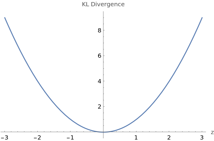
Plot how the Kullback–Leibler divergence varies as the center of the second multinormal distribution moves on a line extended from the origin:
Scope (3)
Compute the Kullback–Leibler divergence of two normal distributions:
Compute the Kullback–Leibler divergence of two binormal distributions:
Compute the Kullback–Leibler divergence symbolically:
Applications (3)
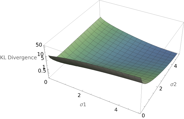
Compare the Kullback–Leibler divergence of two orthogonal multinormal distributions as parameters of their covariance matrices change:
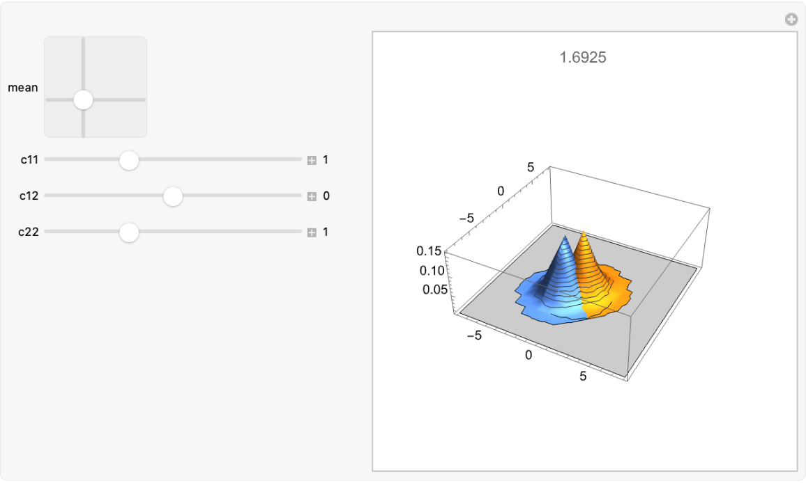
Use a Manipulate to compare two multinormal distributions and show their Kullback–Leibler divergence:
Compute the symbolic Kullback–Leibler divergence for a multinormal distribution with itself, but with the second distribution undergoing a rotation of its covariance matrix:
The same computation, but with a three dimensional multinormal distribution:
Properties and Relations (2)
One can use the more general resource function KullbackLeiblerDivergence, but MultinormalKLDivergence is somewhat faster for low-dimensional distributions:
MultinormalKLDivergence is much faster for higher-dimensional distributions:
Possible Issues (2)
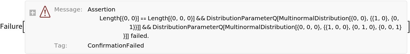
If the two multinormal distributions supplied have different dimensions, a Failure object will result:
If one or more of the distributions is not a multivariate normal distribution, a Failure object will result:
Neat Examples (5)
Use the Kullback–Leibler divergence to help regularization in a variational autoencoder. Create an expression for the Kullback–Leibler divergence between a multinormal distribution with zero mean and a unit, diagonal covariance matrix:
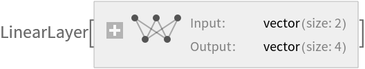
Use the resulting expression to create a function layer that can be used for regularization:
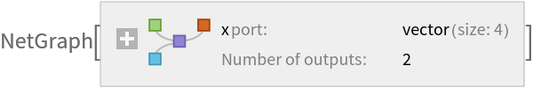
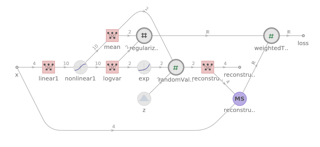
Build a variational autoencoder architecture that uses the Kullback–Leibler divergence to prevent overfitting and to encourage the model to learn a compact and meaningful representation of the data:
Create structured data that one wants the variational autoencoder to capture:
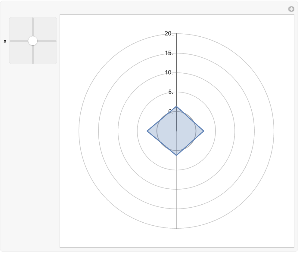
Use a RadialAxisPlot to show the smooth and compact reconstruction of the original vector from a latent space:
![ResourceFunction["MultinormalKLDivergence"][
MultinormalDistribution[{0, 0}, {{1, 1/2}, {1/2, 1/3}}], MultinormalDistribution[{1, 1}, {{1, 1}, {1, 2}}]]](https://www.wolframcloud.com/obj/resourcesystem/images/425/42515a5f-51c8-4b6e-951b-9b761f2afbc4/0f46f1b82a292e20.png)
![Plot[ResourceFunction["MultinormalKLDivergence"][
MultinormalDistribution[{0, 0}, {{1, 0}, {0, 1}}], MultinormalDistribution[{z, z}, {{1, 0}, {0, 1}}]], {z, -3, 3}, AxesLabel -> {"z", "KL Divergence"}]](https://www.wolframcloud.com/obj/resourcesystem/images/425/42515a5f-51c8-4b6e-951b-9b761f2afbc4/554ddcfa2a1bebde.png)

![Plot3D[ResourceFunction["MultinormalKLDivergence"][
MultinormalDistribution[{0, 0}, {{\[Sigma]1, 0}, {0, \[Sigma]1}}], MultinormalDistribution[{1, 1}, {{\[Sigma]2, 0}, {0, \[Sigma]2}}]], {\[Sigma]1, 0.1, 5}, {\[Sigma]2, 0.1, 5}, AxesLabel -> {"\[Sigma]1", "\[Sigma]2", "KL Divergence"}, PlotRange -> All, ScalingFunctions -> "Log", ColorFunction -> "AlpineColors"]](https://www.wolframcloud.com/obj/resourcesystem/images/425/42515a5f-51c8-4b6e-951b-9b761f2afbc4/07db9e49c681feef.png)
![klplot[mean_, c11_, c12_, c22_] := Module[{cv2$ = {{c11, c12}, {c12, c22}}, dist1$ = MultinormalDistribution[{0, 0}, {{1, 0}, {0, 1}}], dist2$,
pd2$}, pd2$ = PositiveDefiniteMatrixQ[cv2$]; If[pd2$, dist2$ = MultinormalDistribution[mean, cv2$]; Plot3D[{PDF[dist1$, {x, y}], PDF[dist2$, {x, y}]}, {x, -8, 8}, {y, -8, 8}, ImageSize -> 300, ImagePadding -> 40, PlotRange -> {0.0001, All}, MaxRecursion -> 5, MeshFunctions -> {#3 &}, PlotLabel -> ResourceFunction["MultinormalKLDivergence"][dist1$, dist2$]], Plot3D[{PDF[dist1$, {x, y}], PDF[dist2$, {x, y}]}, {x, -8, 8}, {y, -8, 8}, ImageSize -> 300, ImagePadding -> 40, PlotRange -> {0.0001, All}, MaxRecursion -> 5, MeshFunctions -> {#3 &}, PlotLabel -> "Covariance matrix of second distribution is not positive definite"]]]](https://www.wolframcloud.com/obj/resourcesystem/images/425/42515a5f-51c8-4b6e-951b-9b761f2afbc4/5e5a807829a295bd.png)
![Manipulate[
klplot[mean, c11, c12, c22], {{mean, {1, 1}}, {-4, -4}, {4, 4}}, {{c11, 1}, 0.1, 3, 0.1, Appearance -> "Labeled"}, {{c12, 0}, -3, 3, 0.1, Appearance -> "Labeled"}, {{c22, 1}, 0.1, 3, 0.1, Appearance -> "Labeled"}, ControlPlacement -> Left]](https://www.wolframcloud.com/obj/resourcesystem/images/425/42515a5f-51c8-4b6e-951b-9b761f2afbc4/2c31b255fb788f84.png)
![ResourceFunction["MultinormalKLDivergence"][
MultinormalDistribution[{0, 0, 0}, {{1, 0, 0}, {0, 1, 0}, {0, 0, 1}}], MultinormalDistribution[{0, 0, 0}, RotationMatrix[\[Theta], {x, y, z}] //. Conjugate[x_] :> x // Simplify]] // FullSimplify[#, {x > 0, y > 0, z > 0}] &](https://www.wolframcloud.com/obj/resourcesystem/images/425/42515a5f-51c8-4b6e-951b-9b761f2afbc4/2a14f2e456dfd896.png)
![n = 20;
cov1 = With[{m = RandomVariate[NormalDistribution[], {n, n}]}, m . Transpose[m]];
cov2 = With[{m = RandomVariate[NormalDistribution[], {n, n}]}, m . Transpose[m]];
dist1 = MultinormalDistribution[
RandomVariate[NormalDistribution[], Length[cov1]], cov1];
dist2 = MultinormalDistribution[
RandomVariate[NormalDistribution[], Length[cov2]], cov2];](https://www.wolframcloud.com/obj/resourcesystem/images/425/42515a5f-51c8-4b6e-951b-9b761f2afbc4/4473ecc9f5407a56.png)
![Quiet@ResourceFunction["MultinormalKLDivergence"][
MultinormalDistribution[{0, 0}, DiagonalMatrix[{1, 1}]], MultinormalDistribution[{#1[[1]], #2[[2]]}, DiagonalMatrix[Exp@{#2[[1]], #2[[2]]}]]] // InputForm](https://www.wolframcloud.com/obj/resourcesystem/images/425/42515a5f-51c8-4b6e-951b-9b761f2afbc4/018dbbc225b43af9.png)
![regularizer = FunctionLayer[
Apply[1/2 (-2 + Exp[#2[[1]]] + Exp[#2[[2]]] - #2[[1]] - #2[[2]] + #1[[1]]^2 + #1[[2]]^2) &]]](https://www.wolframcloud.com/obj/resourcesystem/images/425/42515a5f-51c8-4b6e-951b-9b761f2afbc4/03b1d0107dbc020a.png)

![Information[
net = NetGraph[
Association["linear1" -> LinearLayer[10], "nonlinear1" -> Tanh, "mean" -> LinearLayer[2, "Input" -> 10, "Biases" -> None], "logvar" -> LinearLayer[2, "Input" -> 10, "Biases" -> None], "exp" -> ElementwiseLayer[Exp], "z" -> RandomArrayLayer[NormalDistribution[0, 1] &, "Output" -> 2], "randomValue" -> FunctionLayer[Apply[#1 + #2*#3 &]], "reconstructor" -> LinearLayer[4], "reconstructionLoss" -> MeanSquaredLossLayer[], "regularizationLoss" -> regularizer, "weightedTotalLoss" -> FunctionLayer[Apply[#1 + 0.025*#2 &]]], {NetPort["x"] -> "linear1" -> "nonlinear1" -> {"mean", "logvar"}, "logvar" -> "exp", {"mean", "exp", "z"} -> "randomValue" -> "reconstructor", {"reconstructor", NetPort["x"]} -> "reconstructionLoss", {"mean", "logvar"} -> "regularizationLoss", {"reconstructionLoss", "regularizationLoss"} -> "weightedTotalLoss" -> NetPort["loss"],
"reconstructor" -> NetPort["reconstruction"]}, "x" -> 4, "reconstruction" -> 4], "SummaryGraphic"]](https://www.wolframcloud.com/obj/resourcesystem/images/425/42515a5f-51c8-4b6e-951b-9b761f2afbc4/429d140001156f8e.png)
![self[edgeList_List] := First[Last /@ edgeList];
g1 = Graph[{1, 2, 3, 4}, {1 -> 2, 1 -> 3, 2 -> 4, 3 -> 4}, VertexLabels -> Placed[Automatic, Center], VertexSize -> Large];
SeedRandom[20230211];
initialization1 = 1 -> RandomVariate[DiscreteUniformDistribution[{1, 10}], 100];
functions1 = {x, y, z} |-> Switch[self[z], 2, MapThread[
v |-> RandomVariate[DiscreteUniformDistribution[{v, v + 3}]], x],
3, MapThread[v |-> RandomVariate[NormalDistribution[v, 1]], x], 4, MapThread[{v1, v2} |-> RandomVariate[NormalDistribution[2 v1 - v2, 1]], x]];](https://www.wolframcloud.com/obj/resourcesystem/images/425/42515a5f-51c8-4b6e-951b-9b761f2afbc4/0a8e042ccb90a7a5.png)
![(x = Thread[Values[ResourceFunction[
ResourceObject[<|"Name" -> "DirectedAcyclicEvaluate", "ShortName" -> "DirectedAcyclicEvaluate", "UUID" -> "6a982fd7-4993-4495-aced-a4d53a852dbc", "ResourceType" -> "Function", "Version" -> "1.1.0", "Description" -> "Evaluate functions locally over any directed acyclic graph", "RepositoryLocation" -> URL[
"https://www.wolframcloud.com/obj/resourcesystem/api/1.0"],
"SymbolName" -> "FunctionRepository`$870b98ec382e4ca2b7fe695c0e6142f1`DirectedAcyclicEvaluate", "FunctionLocation" -> CloudObject[
"https://www.wolframcloud.com/obj/37c15cca-bccf-4865-9565-5921a229f8d6"]|>, ResourceSystemBase -> Automatic]][g1, initialization1, functions1][["VertexWeights"]]]]) // Short](https://www.wolframcloud.com/obj/resourcesystem/images/425/42515a5f-51c8-4b6e-951b-9b761f2afbc4/045feff73eecc29c.png)