Function Repository Resource:

TimeShiftedDistribution

A derived distribution useful in actuarial science

Contributed by: Seth J. Chandler

ResourceFunction["TimeShiftedDistribution"][x_min,dist]

represents a distribution dist that has been truncated to lie above x_min and then translated so that the lowest outcome is 0.

ResourceFunction["TimeShiftedDistribution"][{x_min,y_min,…},dist]

represents a multivariate truncation of the distribution dist, translated so the lowest outcome from the distribution is a vector of 0s.

Details and Options

The translation works by subtracting x_min from the outputs so that the lowest outcome from the distribution is now 0.

A time-shifted distribution can be used to model the longevity of a person who had a certain longevity distribution at birth but who has survived to some attained age.

Examples

Basic Examples (2)

A BinomialDistribution, time-shifted so that its value must lie above 3 and be translated to the left by 3:

In[1]:=

Out[1]=

The probability density (mass) function of that distribution:

In[2]:=

Out[3]=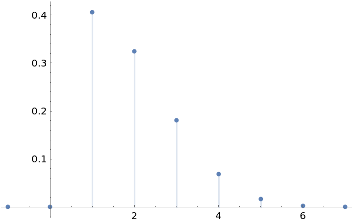

The distribution of the remaining life of a person aged 61, where longevity at birth is distributed according to a GompertzMakehamDistribution:

In[4]:=

Out[4]=

The survival function of that time-shifted distribution:

In[5]:=

Out[5]=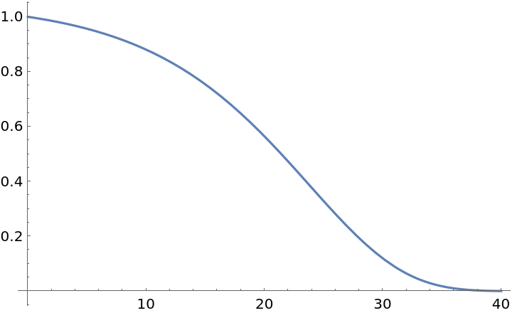

Scope (2)

The mean of a time-shifted distribution of a ProductDistribution of two symbolic BetaDistributions:

In[6]:=

TraditionalForm@
Refine[Mean@
ResourceFunction["TimeShiftedDistribution"][{x, y}, ProductDistribution[BetaDistribution[a1, b1], BetaDistribution[a2, b2]]], {0 < x < 1, 0 < y < 1}]

Out[6]=

A random variable drawn from a time-shifted MultinormalDistribution:

In[7]:=

Out[7]=

The numeric probability of a draw from a time-shifted CopulaDistribution falling into a particular set of values:

In[8]:=

$NProbability[ 0 < x < 2 && y > 0.3, {x, y} \[Distributed] ResourceFunction["TimeShiftedDistribution"][{2, 2}, CopulaDistribution[{"Binormal", -0.3}, {NormalDistribution[0, 1], NormalDistribution[0.5, 0.7]}]] ]$

Out[8]=

Applications (2)

Show survival functions of a BetaDistribution for different time-shift values:

In[9]:=

$With[{survivalFunctions = Table[SurvivalFunction[ ResourceFunction["TimeShiftedDistribution"][t, BetaDistribution[3, 3]], x], {t, Range[0, 0.8, 0.1]}]}, Plot[survivalFunctions, {x, 0, 1}, PlotLabel -> "Time Shifted Survival Functions\nof a Beta Distribution", PlotLegends -> Placed[LineLegend[Range[0, 0.8, 0.1], LegendLabel -> "Time Shift"], Bottom]]]$

Out[9]=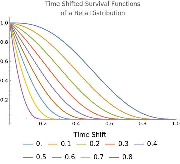

Show survival functions of a GompertzMakehamDistribution for different time-shift values:

In[10]:=

$With[{survivalFunctions = Table[SurvivalFunction[ ResourceFunction["TimeShiftedDistribution"][t, GompertzMakehamDistribution[1/8, 1/40000]], x], {t, Range[0, 90, 10]}]}, Plot[survivalFunctions, {x, 0, 100}, PlotLabel -> "Time Shifted Survival Functions\nof a Gompertz-Makeham Distribution", PlotLegends -> Placed[LineLegend[Range[0, 90, 10], LegendLabel -> "Time Shift"], Bottom]]]$

Out[10]=

Properties and Relations (1)

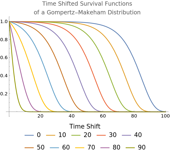Some distributions, such as the ExponentialDistribution, remain unchanged after time shifting :

In[11]:=

$CDF[ExponentialDistribution[\[Lambda]], x] - CDF[ResourceFunction["TimeShiftedDistribution"][t, ExponentialDistribution[\[Lambda]]], x] // Simplify[#, {x > 0, t > 0}] &$

Out[11]=

Neat Examples (3)

Consider a life insurance product in which the time a person dies and the time a person lets their policy lapse are given by the ProductDistribution of a GompertzMakehamDistribution (for longevity) and an ExponentialDistribution (for lapse). The insured has neither died nor lapsed before age 61. Compute the probability that an insurer will have to pay a death benefit between k and k+1 years thereafter and that the insurance policy will not have lapsed by that time:

In[12]:=

In[13]:=

Out[13]=

In[14]:=

$FullSimplify[ Probability[ k < death < k + 1 && lapse > k + 1, {death, lapse} \[Distributed] deathLapseDistribution61], k > 0]$

Out[14]=

Compute the actuarial present value of a death benefit of $1 for such a person, assuming the policy pays nothing if the policy lapses before death and assuming a 5% effective rate of interest:

In[15]:=

$NExpectation[ If[death < lapse, 1/(1 + 0.05)^death, 0], {death, lapse} \[Distributed] deathLapseDistribution61]$

Out[15]=

Compute the maximum amount the insurer would be willing to pay a 75-year-old who holds such a policy to let it lapse, again assuming a 5% effective rate of interest:

In[16]:=

$NExpectation[ If[death < lapse, 1/(1 + 0.05)^death, 0], {death, lapse} \[Distributed] ResourceFunction["TimeShiftedDistribution"][{75, 75}, ProductDistribution[GompertzMakehamDistribution[1/8, 1/40000], ExponentialDistribution[3/10]]]]$

Out[16]=

Publisher

Seth J. Chandler

Version History

1.0.0 – 07 August 2019

Source Metadata

Citation:
- Promislow, S. D., Fundamentals of Actuarial Mathematics, 3rd edition. Chichester: John Wiley & Sons, 2015.

Related Resources

License Information

This work is licensed under a Creative Commons Attribution 4.0 International License