Function Repository Resource:

MultisetSokalSneathDissimilarity

Source Notebook

Compute the Sokal-Sneath dissimilarity of two multisets

Contributed by: Robert B. Nachbar (Wolfram Solutions)

ResourceFunction["MultisetSokalSneathDissimilarity"][list1,list2]

gives the Sokal–Sneath dissimilarity between multisets list1 and list2.

ResourceFunction["MultisetSokalSneathDissimilarity"][assoc1,assoc2]

gives the Sokal–Sneath dissimilarity between multisets assoc1 and assoc2.

Details and Options

If the listi are considered as multisets, ResourceFunction["MultisetSokalSneathDissimilarity"] gives their dissimilarity.
The listi must have the same head, but it need not be List.
The values of associ must be counts—that is, non-negative Integer values.
ResourceFunction["MultisetSokalSneathDissimilarity"][A,B] is equivalent to .

Examples

Basic Examples (2) 

Sokal-Sneath dissimilarity between two List multisets:

In[1]:=
ResourceFunction[
 "MultisetSokalSneathDissimilarity"][{"a", "c"}, {"a", "b"}]
Out[1]=

Sokal-Sneath dissimilarity between two Association multisets:

In[2]:=
ResourceFunction[
 "MultisetSokalSneathDissimilarity"][<|"a" -> 1, "c" -> 1, "d" -> 1|>, <|"a" -> 1, "b" -> 1, "d" -> 1, "e" -> 1|>]
Out[2]=

Scope (1) 

The number of elements of each distinct kind affects the result:

In[3]:=
ResourceFunction[
 "MultisetSokalSneathDissimilarity"][{"a", "a", "b", "c", "c", "c"}, {"a", "b", "c"}]
Out[3]=
In[4]:=
ResourceFunction[
 "MultisetSokalSneathDissimilarity"][{"a", "a", "b", "c", "c", "c"}, {"a", "b", "b", "b", "c"}]
Out[4]=
In[5]:=
ResourceFunction[
 "MultisetSokalSneathDissimilarity"][<|"a" -> 1, "b" -> 2, "c" -> 3|>, <|"a" -> 2, "b" -> 3, "c" -> 1|>]
Out[5]=
In[6]:=
ResourceFunction[
 "MultisetSokalSneathDissimilarity"][<|"a" -> 1, "b" -> 2, "c" -> 3|>, <|"a" -> 2, "b" -> 2, "c" -> 2|>]
Out[6]=

Applications (22) 

The Sokal-Sneath dissimilarity measure has its origins in numerical taxonomy. It was proposed by Robert R. Sokal and Peter H. A. Sneath as a measure of similarity in the same class as the Jaccard and Dice measures but with an alternative weighting of unmatched features.

The measure can be used in a number of fields, as shown by the following examples. The role of object and attribute can also be reversed, and the first application demonstrates this duality.

Ecology (5) 

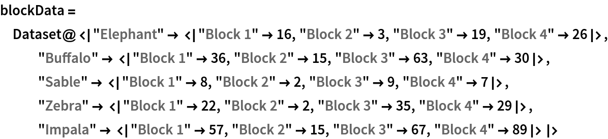
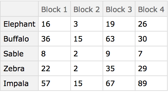
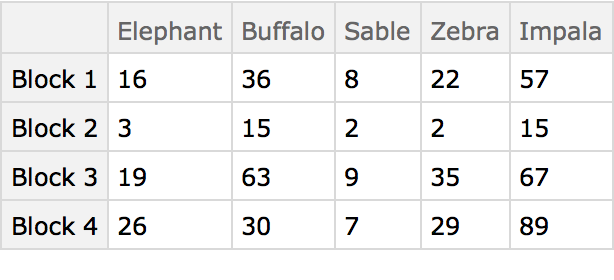
Here are some ground-based animal index counts:

In[7]:=
blockData = Dataset@<|"Elephant" -> <|"Block 1" -> 16, "Block 2" -> 3, "Block 3" -> 19, "Block 4" -> 26|>, "Buffalo" -> <|"Block 1" -> 36, "Block 2" -> 15, "Block 3" -> 63, "Block 4" -> 30|>, "Sable" -> <|"Block 1" -> 8, "Block 2" -> 2, "Block 3" -> 9, "Block 4" -> 7|>, "Zebra" -> <|"Block 1" -> 22, "Block 2" -> 2, "Block 3" -> 35, "Block 4" -> 29|>, "Impala" -> <|"Block 1" -> 57, "Block 2" -> 15, "Block 3" -> 67, "Block 4" -> 89|>|>
Out[7]=

Here the different blocks (habitats) are compared using the animals present as characters. The arrangement of the table in this manner originated in the field of psychology, and was later adopted by numerical taxonomy.

The MultisetSokalSneathDissimilarity distance matrix of the blocks:

In[8]:=
DistanceMatrix[Values@Transpose@blockData, DistanceFunction -> ResourceFunction[
   "MultisetSokalSneathDissimilarity"]] // Row[{MatrixForm@#, MatrixForm@N@#}, Spacer[18]] &
Out[8]=

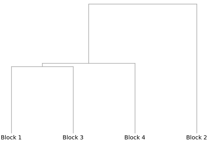
A Dendrogram showing how the blocks cluster:

In[9]:=
Dendrogram[Normal@Transpose@blockData, DistanceFunction -> ResourceFunction[
  "MultisetSokalSneathDissimilarity"]]
Out[9]=

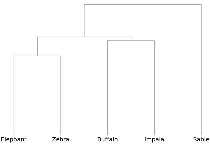
The preceding analysis that compares the columns of the table is known as a Q-type (deriving from early factor analysis studies in the area of psychology). Conversely, comparing the rows is known as an R-type analysis and in this case compares the animals. Begin by first transposing the data table:

In[10]:=
speciesData = Dataset@Normal@Transpose@blockData
Out[10]=

A Dendrogram shows that elephants and zebras, for example, are distributed similarly:

In[11]:=
Dendrogram[Normal@Transpose@speciesData, DistanceFunction -> ResourceFunction[
  "MultisetSokalSneathDissimilarity"]]
Out[11]=

Taxonomy (3) 

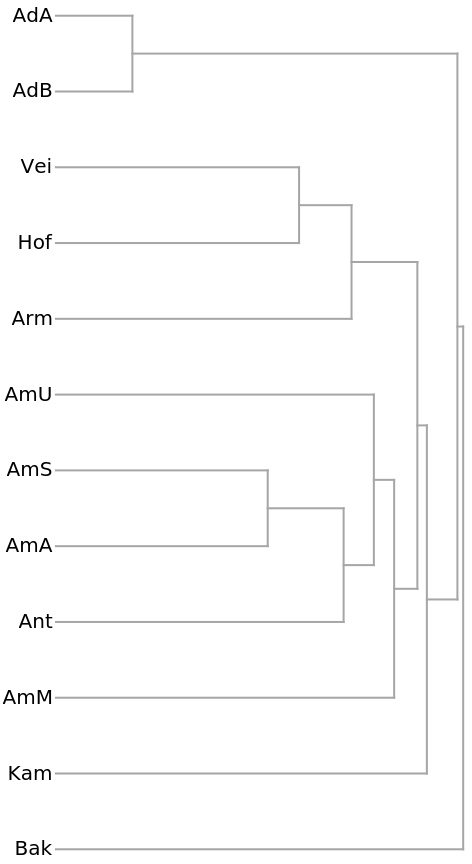
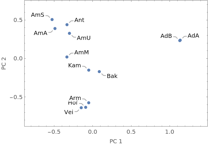
This application uses the chemical composition of flower parts from Hawaiian anthurium plants to classify different species and commercial cultivars. Load the data:

In[12]:=
data = {{"Compound ID \\ Species", "AdA", "AdB", "AmU", "AmS", "AmM", "AmA", "Ant", "Arm", "Bak", "Hof", "Kam", "Vei"}, {"1", 626, 615, 1, 0, 2, 1, 0, 0, 0, 0, 9, 0}, {"2", 13, 16, 283, 136, 68, 151, 5,
     0, 0, 0, 921, 0}, {"3", 0, 0, 48, 21, 33, 22, 2, 0, 0, 0, 7, 0}, {"4", 3689, 3338, 0, 3, 26, 1, 3, 1, 0, 0, 0, 0}, {"5", 0, 0, 0, 0, 0, 0, 0, 0, 0, 0, 0, 0}, {"6", 39, 1, 0, 0, 0, 0, 0, 0, 0, 0, 0, 0}, {"7", 0, 0, 1626, 824, 184, 428, 719, 0, 0, 0, 0, 0}, {"8", 9, 8, 0, 0, 0, 0, 0, 20, 0, 0, 0, 0}, {"9", 1900, 1720, 323, 244, 244, 198, 112, 349, 89, 438, 252, 334}, {"10", 0, 0, 0, 0, 0, 0, 84, 0, 0, 0, 0, 0}, {"11", 0, 0, 39, 18, 4, 5, 0, 0, 0, 0, 0, 0}, {"12", 0, 0, 0, 0, 0, 0, 72, 0, 0, 0, 0, 0}, {"13", 0, 0, 0, 0, 0, 0, 0, 0, 408, 0, 0, 0}, {"14", 0, 0, 21, 12, 7, 11, 0,
     0, 0, 0, 0, 0}, {"15", 0, 0, 0, 0, 0, 0, 7, 0, 0, 0, 0, 0}, {"16", 0, 0, 0, 0, 190, 0, 25, 0, 0, 70, 0, 0}, {"17", 0, 0, 0, 0, 0, 0, 0, 0, 0, 0, 0, 0}, {"18", 0, 0, 0, 0, 0, 0, 33, 0, 0, 0, 0, 0}, {"19", 0, 0, 62, 18, 35, 18, 23, 1, 0, 4, 92, 4}, {"20",
     0, 0, 0, 0, 0, 0, 0, 26, 0, 0, 0, 0}, {"21", 0, 0, 0, 0, 0, 0, 0,
     8, 0, 115, 0, 0}, {"22", 0, 0, 0, 0, 0, 0, 0, 0, 0, 0, 469, 0}, {"23", 4, 6, 0, 0, 0, 0, 0, 0, 0, 0, 0, 0}, {"24", 0, 0, 16, 8, 18, 5, 2, 0, 0, 0, 0, 0}, {"25", 144, 59, 0, 0, 0, 0, 0, 0, 0, 0, 0, 0}, {"26", 0, 0, 0, 0, 0, 0, 12, 13, 0, 0, 0, 0}, {"27", 0, 0, 0, 0, 0, 0, 0, 2, 0, 0, 0, 0}, {"28", 0, 0, 0, 0, 0, 0, 0, 0, 0, 0, 0, 6}, {"29", 6, 7, 0, 0, 0, 0, 0, 2, 0, 0, 13, 7}, {"30", 22, 18, 0, 0, 0, 0, 0, 0, 1, 0, 0, 0}, {"31", 59, 65, 0, 0, 0, 0, 1, 66, 0, 0, 0, 0}, {"32", 1, 0, 139, 0, 9, 3, 0, 0, 0, 0, 0, 0}, {"33", 24, 21, 0, 0, 0, 0, 4, 0, 0, 0, 0, 0}, {"34", 0, 0, 0, 0, 0, 0, 3, 0, 0, 0, 0, 0}, {"35", 0, 0, 0, 0, 0, 0, 10, 0, 0, 0, 0, 0}, {"36", 2, 0, 2, 0, 0, 0, 0, 405, 0, 0, 0, 0}, {"37", 2, 1, 0, 0, 0, 0, 0, 28, 0, 0, 0, 0}, {"38", 0, 0, 0, 0, 0, 0, 26, 0, 0,
     0, 0, 71}, {"39", 51, 10, 0, 0, 0, 0, 0, 0, 0, 0, 0, 0}, {"40", 723, 689, 166, 139, 133, 114, 67, 205, 37, 265, 126, 214}, {"41", 235, 238, 74, 64, 56, 56, 26, 98, 2, 135, 95, 105}, {"42", 103, 89, 9, 2, 12, 4, 35, 43, 6, 28, 28, 12}};
In[13]:=
TableForm[data[[2 ;; 9, ;; 8]], TableHeadings -> {None, data[[1, ;; 8]]}]
Out[13]=
In[14]:=
taxonomicData = With[{species = Rest@First@data, amounts = Thread[First@# -> Rest@#] & /@ Rest@data}, MapThread[#1 -> DeleteCases[Association@#2, 0] &, {species, Transpose@amounts}]];
Short@%
Out[10]=

A Dendrogram shows the clustering of the species:

In[15]:=
Dendrogram[Association@taxonomicData, Right, DistanceFunction -> ResourceFunction[
  "MultisetSokalSneathDissimilarity"], ClusterDissimilarityFunction -> "Average"]
Out[15]=

A feature space plot can be made from the PrincipalComponents of the distance matrix:

In[16]:=
With[{species = Keys@taxonomicData, prinComp = Take[#, 2] & /@ PrincipalComponents[
     1 - N@DistanceMatrix[Values@taxonomicData, DistanceFunction -> ResourceFunction[
         "MultisetSokalSneathDissimilarity"]]]},
 ListPlot[MapThread[Callout, {prinComp, species}], FrameLabel -> {"PC 1", "PC 2"}, PlotRange -> All, PlotRangePadding -> Scaled[0.15], AspectRatio -> Automatic]
 ]
Out[16]=

Sociology (6) 

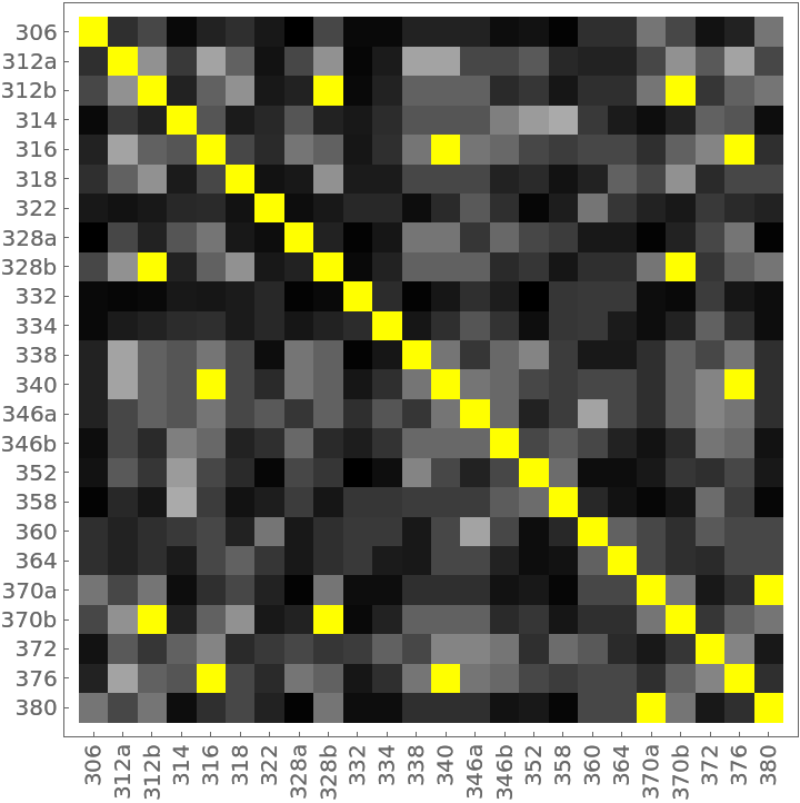
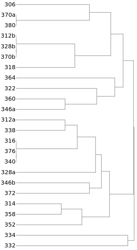
This example compares households on a single city block using the composition of household members (head, wife, daughter, brother-in-law, etc.). The data was compiled from the 1920 US Census for the 300 block of Wyoming Ave., Buffalo, NY. The households are labeled by street number.

Load the data:

In[17]:=
data = <|"306" -> {"head", "wife", "step-son"}, "312a" -> {"head", "wife", "son", "son"}, "312b" -> {"head", "wife", "son"}, "314" -> {"head", "wife", "daughter", "son", "son", "son", "son", "daughter", "son"}, "316" -> {"head", "wife", "son", "daughter", "son"}, "318" -> {"head", "wife", "son", "mother-in-law"}, "322" -> {"head", "wife", "daughter", "daughter", "niece", "niece"},
    "328a" -> {"head", "son", "son", "daughter", "son"}, "328b" -> {"head", "wife", "son"}, "332" -> {"head", "wife", "daughter", "daughter", "daughter", "daughter", "daughter", "brother-in-law", "mother-in-law"}, "334" -> {"head", "wife", "daughter", "son", "daughter", "daughter", "grandson", "grandson", "grandson"}, "338" -> {"head", "wife", "son", "son", "son"}, "340" -> {"head", "wife", "son", "son", "daughter"}, "346a" -> {"head", "wife", "son", "daughter", "daughter"}, "346b" -> {"head", "wife", "son", "son", "daughter", "daughter", "son", "sister"}, "352" -> {"head", "wife", "son", "son", "son", "son", "son"}, "358" -> {"head", "wife", "daughter", "son", "daughter", "son", "daughter", "daughter", "son", "son", "son"}, "360" -> {"head", "wife", "daughter", "daughter"}, "364" -> {"head", "wife", "daughter", "mother-in-law"}, "370a" -> {"head", "wife"}, "370b" -> {"head", "wife", "son"}, "372" -> {"head", "wife", "daughter", "daughter", "daughter", "son", "son"}, "376" -> {"head", "wife", "son", "son", "daughter"}, "380" -> {"head", "wife"}|>;
RandomSample[%, 3]
Out[13]=

The aggregate composition of the neighborhood:

In[18]:=
Join @@ Values@data // Counts // KeySort
Out[18]=

The distance matrix using MultisetDiceDissimilarity can be displayed with an ArrayPlot (note the presence of off-diagonal 0s colored yellow):

In[19]:=
With[{labels = Keys@data}, DistanceMatrix[Values@data, DistanceFunction -> ResourceFunction[
    "MultisetSokalSneathDissimilarity"]] // ArrayPlot[#, FrameTicks -> {Thread[{Range@Length@labels, labels}], Thread[{Range@Length@labels, Rotate[#, 90 °] & /@ labels}]}, ColorRules -> {0 -> Yellow}] &]
Out[19]=

The clustering of the households as shown by a Dendrogram:

In[20]:=
Dendrogram[data, Right, DistanceFunction -> ResourceFunction[
  "MultisetSokalSneathDissimilarity"], ClusterDissimilarityFunction -> "Average"]
Out[20]=

The 14 yellow-colored, off-diagonal 0s of the preceding distance matrix represent pairs of identical households. They also appear in the preceding dendrogram as leaves with no initial height. Here they are extracted as clusters:

In[21]:=
clusters = ClusteringTree[data, 0, DistanceFunction -> ResourceFunction[
     "MultisetSokalSneathDissimilarity"], ClusterDissimilarityFunction -> "Average"] // PropertyValue[#, "LeafLabels"] &;
In[22]:=
identicalHousholds = Select[clusters, Length[#] > 1 &] // Values
Out[22]=

Finally, mapping back to the original household data gives:

In[23]:=
Function[cluster, KeySelect[data, MemberQ[cluster, #] &]] /@ identicalHousholds
Out[23]=

Economics (3) 

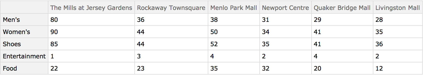
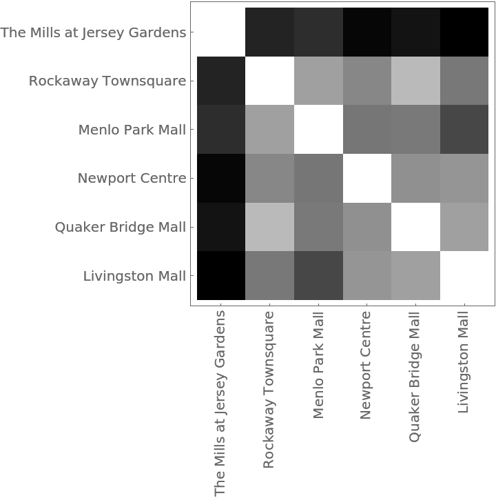
Understanding market forces and characteristics of the competition are essential components of profitable business decisions. This example shows how shopping malls might be compared using the numbers of kinds of businesses in each. The data was collected from the websites of each mall using the self-reported number of businesses in each category. These malls are all managed by the same organization, so the categories can be assumed to be consistent.

Load the data:

In[24]:=
data = Dataset[<|"Men's" -> <|"The Mills at Jersey Gardens" -> 80, "Rockaway Townsquare" -> 36, "Menlo Park Mall" -> 38, "Newport Centre" -> 31, "Quaker Bridge Mall" -> 29, "Livingston Mall" -> 28|>, "Women's" -> <|"The Mills at Jersey Gardens" -> 90, "Rockaway Townsquare" -> 44, "Menlo Park Mall" -> 50, "Newport Centre" -> 34, "Quaker Bridge Mall" -> 41, "Livingston Mall" -> 35|>, "Shoes" -> <|"The Mills at Jersey Gardens" -> 85, "Rockaway Townsquare" -> 44, "Menlo Park Mall" -> 52, "Newport Centre" -> 35, "Quaker Bridge Mall" -> 41, "Livingston Mall" -> 36|>, "Entertainment" -> <|"The Mills at Jersey Gardens" -> 1, "Rockaway Townsquare" -> 3, "Menlo Park Mall" -> 4, "Newport Centre" -> 2, "Quaker Bridge Mall" -> 4, "Livingston Mall" -> 2|>, "Food" -> <|"The Mills at Jersey Gardens" -> 22, "Rockaway Townsquare" -> 23, "Menlo Park Mall" -> 35, "Newport Centre" -> 32, "Quaker Bridge Mall" -> 20, "Livingston Mall" -> 12|>|>, 
TypeSystem`Assoc[
TypeSystem`Atom[String], 
TypeSystem`Struct[{"The Mills at Jersey Gardens", "Rockaway Townsquare", "Menlo Park Mall", "Newport Centre", "Quaker Bridge Mall", "Livingston Mall"}, {
TypeSystem`Atom[Integer], 
TypeSystem`Atom[Integer]}], 5], <|"ID" -> 85792143290300|>]
Out[24]=

The distance matrix using MultisetDiceDissimilarity can be displayed with an ArrayPlot:

In[25]:=
With[{labels = Normal@Keys@Transpose@data}, DistanceMatrix[Values@Transpose@data, DistanceFunction -> ResourceFunction[
    "MultisetSokalSneathDissimilarity"]] // ArrayPlot[#, FrameTicks -> {Thread[{Range@Length@labels, labels}], Thread[{Range@Length@labels, Rotate[#, 90 °] & /@ labels}]}] &]
Out[25]=

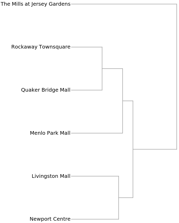
The Dendrogram shows that The Mills at Jersey Gardens is very different from the others:

In[26]:=
Dendrogram[Normal@Transpose@data, Right, DistanceFunction -> ResourceFunction[
  "MultisetSokalSneathDissimilarity"], ClusterDissimilarityFunction -> "Average"]
Out[26]=

Chemistry (5) 

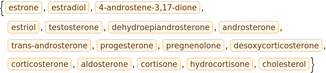
Similarity analysis of chemical structures goes back to the original work of Carhart et al. at Lederle Laboratories. It is used extensively to search though chemical databases to find compounds of interest and to cluster chemical structures into similar groups.

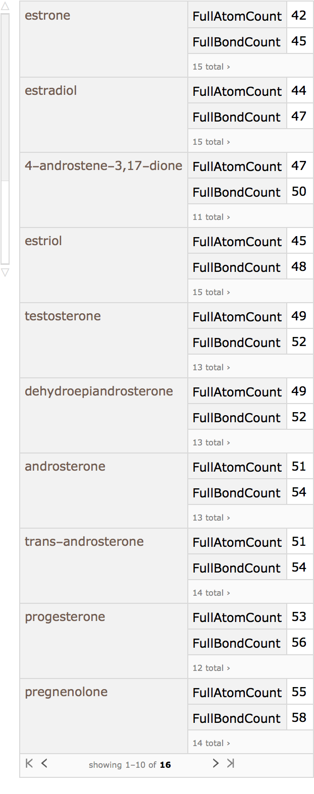
Here is small set of entities from the ChemicalData collection:

In[27]:=
molNames = ChemicalData[EntityClass["Chemical", "Steroids"]]
Out[27]=

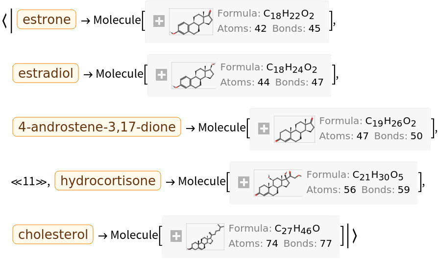
They can be converted into computable Molecule objects:

In[28]:=
mols = # -> Molecule@# & /@ molNames // Association;
Short@%
Out[26]=

These are the topological features that will characterize each chemical structure (they are not the same as those used by Carhart et al., but are easily computable with MoleculeValue):

In[29]:=
properties = {"FullAtomCount", "FullBondCount", "AliphaticCarbocycleCount", "AliphaticHeterocycleCount", "AliphaticRingCount", "AmideBondCount", "AromaticCarbocycleCount", "AromaticHeterocycleCount", "AromaticRingCount", "BridgeheadAtomCount", "HBondAcceptorCount", "HBondDonorCount", "HeteroatomCount", "HeterocycleCount", "LipinskiHBondAcceptorCount", "LipinskiHBondDonorCount", "RingCount", "RotatableBondCount", "SaturatedCarbocycleCount", "SaturatedHeterocycleCount", "SaturatedRingCount", "SpiroAtomCount", "StereocenterCount", "UnspecifiedStereocenterCount"};

Using Dataset, a searchable database can be made:

In[30]:=
database = Dataset@(DeleteCases[#, 0] &@
      AssociationThread[
       properties -> MoleculeValue[#, properties]] & /@ mols)
Out[30]=

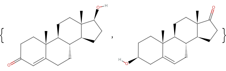
Testosterone, for example, can be taken as the query molecule:

In[31]:=
queryMolecule = Normal@database[Entity["Chemical", "Testosterone"]]
Out[31]=
In[32]:=
hits = Query[
    Select[ResourceFunction["MultisetSokalSneathDissimilarity"][
         queryMolecule, #] <= 0.05 &]/*Keys]@database // Normal
Out[32]=
In[33]:=
MoleculePlot /@ (hits /. mols)
Out[33]=

Properties and Relations (2) 

Sokal-Sneath dissimilarity is bounded by 0 and 1:

In[34]:=
ResourceFunction[
 "MultisetSokalSneathDissimilarity"][{"a", "c", "c", "d"}, {"a", "c", "c", "d"}]
Out[34]=
In[35]:=
ResourceFunction[
 "MultisetSokalSneathDissimilarity"][{"a", "c", "c", "d"}, {"X", "Y", "Z"}]
Out[35]=

The result is the same as SokalSneathDissimilarity when the multisets are sets:

In[36]:=
ResourceFunction[
 "MultisetSokalSneathDissimilarity"][<|"a" -> 1, "c" -> 1, "d" -> 1|>, <|"a" -> 1, "b" -> 1, "d" -> 1, "e" -> 1|>]
Out[36]=
In[37]:=
SokalSneathDissimilarity[{1, 0, 1, 1, 0}, {1, 1, 0, 1, 1}]
Out[37]=

Publisher

Robert Nachbar

Version History

  • 1.0.0 – 01 July 2019

Source Metadata

Related Resources

License Information