Basic Examples (3)
Eliminate {x,y} from three polynomials to obtain conditions on the coefficient parameter, a, for which the polynomials simultaneously vanish:
We can find the specific values of a for which the three polynomials can simultaneously vanish in {x,y}:
Checking reveals that all but the last two values for a give rise to solutions in {x,y}:
Scope (1)
Here are two polynomials that vanish at x=1:
Options (1)
Use the Dixon resultant modulo 127 to eliminate four variables from a system of five polynomials (example is taken from reference by Tang and Feng):
Possible Issues (2)
Dixon resultant computations involve symbolic row reduction and computation of determinants, and this can be slow (example is from Feng and Li reference):
The result is a polynomial that eliminates the variables {b,d} from the system and it is not small:
Here is a substantially more difficult example:
It is easy to obtain a resultant when numerical values are substituted for parameters:
Obtaining the parametrized resultant takes far longer:
This result is big:
Properties and Relations (2)
Resultants can be used to recover the usual "discriminant" from school algebra, though with an extraneous factor (to account for the possibility of the leading term vanishing):
For two polynomials the Dixon resultant agrees with the usual resultant except perhaps for multiplicities of extraneous factors:
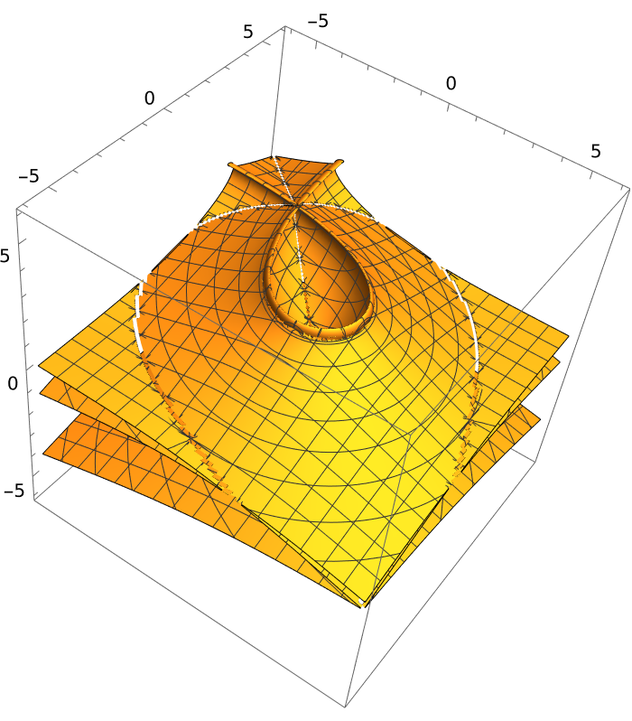
Define a polynomial surface implicitization problem (example is from the Tran reference):
Calculate the Dixon resultant:
A Groebner basis can also be used to eliminate variables; this example requires some non-default settings as well as a numeric-to-exact conversion in order to be at all efficient:
These agree up to a multiplicative constant (so there are no extraneous factors in the Dixon resultant in this example):
Applications (4)
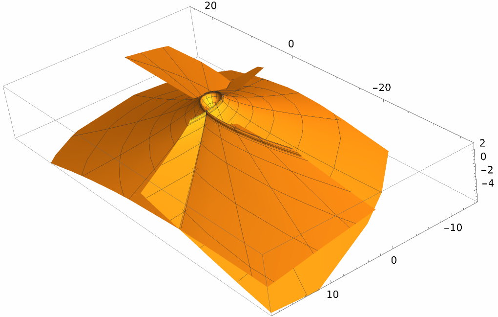
One common use of these resultants is to find the implicit form of a parametrized surface. We illustrate using two parametrized bicubic patches from the Newell (or Utah) Teapot. One gives an easy problem, whereas the other is more challenging:
Plot this surface:
Here is the plot of the original parametrized form:
The second patch above is more difficult to put into implicit form:


![polys = {9 x1 + 37 x3 + 17 x1 x2 + 120 x2 x3 + 18 x3 x5 + 58 x4^2 + 87,
46 x1 + 43 x3 + 117 x5 + 43 x1 x2 + 93 x1 x3 + 61 x3 x4 + 48,
32 x1 x2 + 54 x1 x4 + 56 x2 x3 + 93 x3 x5 + 60 x5^2 + 45,
124 x1 + 93 x1 x3 + 78 x1 x4 + 45 x1 x5 + 39 x2 x3 + 38 x2 x4 + 46,
27 x2 + 95 x2 x5 + 85 x3^2 + 74 x3 x4 + 46 x3 x5 + 77 x4 x5 + 66
};
Timing[dixres = ResourceFunction[
"DixonResultant", ResourceSystemBase -> "https://www.wolframcloud.com/obj/resourcesystem/api/1.0"][polys, {x1, x2, x3, x4}, Modulus -> 127]]](https://www.wolframcloud.com/obj/resourcesystem/images/363/3636f5e3-94e9-46e5-9b3c-79002b586aac/6008653463d85b6f.png)

![polys = {-99 d^2 + 90 d^4 + 86 d^4 b - 84 b f^4 + 8 m^2 d^2 n b - 10 n b^3 f,
78 m n + 34 m b + 66 m - 53 d b + 59 b^2 + 28 b f,
-79 m b + 53 n m^2 + 63 m^2 b - 24 n^3 - 29 d^2 f - 4 d b^2
};
Timing[dixres = ResourceFunction[
"DixonResultant", ResourceSystemBase -> "https://www.wolframcloud.com/obj/resourcesystem/api/1.0"][polys, {b, d}];]](https://www.wolframcloud.com/obj/resourcesystem/images/363/3636f5e3-94e9-46e5-9b3c-79002b586aac/0b306b4a950c1976.png)

![Timing[res = ResourceFunction[
"DixonResultant", ResourceSystemBase -> "https://www.wolframcloud.com/obj/resourcesystem/api/1.0"][
polys /. {c12 -> 2/3, c23 -> -1/2, c34 -> 1/2, c41 -> -3/4, b1 -> 7/3, b2 -> 11/5, b3 -> 9/7, b4 -> 2/11}, {x2, x3, x4}]]](https://www.wolframcloud.com/obj/resourcesystem/images/363/3636f5e3-94e9-46e5-9b3c-79002b586aac/14aa92fe81167c6f.png)


![Timing[gbT = GroebnerBasis[TranPolys, vars, elims, Sort -> True, MonomialOrder -> EliminationOrder, CoefficientDomain -> InexactNumbers[1000], Method -> {"GroebnerWalk", "EarlyEliminate" -> True}];]](https://www.wolframcloud.com/obj/resourcesystem/images/363/3636f5e3-94e9-46e5-9b3c-79002b586aac/36e77a58f59cfac2.png)

![d = 4;
ParametricPlot3D[{-(-(7/5) + (231 s^2)/125 - (56 s^3)/125 + (3 t)/
16 - (99 s^2 t)/400 + (3 s^3 t)/50 - (39 t^2)/80 + (
1287 s^2 t^2)/2000 - (39 s^3 t^2)/250 + t^3/5 - (33 s^2 t^3)/
125 + (8 s^3 t^3)/125), -((294 s)/125 - (63 s^2)/125 - (56 s^3)/
125 - (63 s t)/200 + (27 s^2 t)/400 + (3 s^3 t)/50 + (819 s t^2)/
1000 - (351 s^2 t^2)/2000 - (39 s^3 t^2)/250 - (42 s t^3)/125 + (
9 s^2 t^3)/125 + (8 s^3 t^3)/125), -(-(12/5) - (63 t)/160 + (
63 t^2)/160)}, {s, -2 d/3, 2 d/3}, {t, -d, d}, PlotPoints -> 10]](https://www.wolframcloud.com/obj/resourcesystem/images/363/3636f5e3-94e9-46e5-9b3c-79002b586aac/156e9cf1e06ccd04.png)