Function Repository Resource:

LindbladSolve

Solve the Lindblad master equation

Contributed by: Mohammad Bahrami and Nikolay Murzin

ResourceFunction["LindbladSolve"][h,{L₁,L₂,…,L_m},s,t]

gives the symbolic solution to the Lindblad master equation with the independent variable t, the Hamiltonian h, Lindblad operators L_j and the initial state s.

ResourceFunction["LindbladSolve"][h,{L₁,L₂,…,L_m},s,{t,t_min,t_max}]

gives the numerical solution to the Lindblad master equation with the independent variable t in the range t_min to t_max.

Details and Options

ResourceFunction["LindbladSolve"] gives the solution to the Lindblad master equation

with ρ the density operator, H the Hamiltonian, and L_j the Lindblad operators (also called jump operators).

The Hamiltonian and all Lindblad operators should have the same dimensions.

The initial state can be a vector (pure state) or a density matrix. The solution is given always as a density matrix.

The Lindblad master equation can be also written like

with γ_j the jump rates. One needs to feed the Lindblad operators as

into LindbladSolve in order to get the solution.

ResourceFunction["LindbladSolve"] gives the solution either numerically or symbolically, depending on the inputs.

ResourceFunction["LindbladSolve"] accepts all options of DSolve or NDSolve.

If a range for the independent variable is given, ResourceFunction["LindbladSolve"] gives the numerical solution unless one imposes a symbolic solution by setting Method as "Symbolic".

Method

Automatic

if set as "Symbolic",DSolve will be used to solve the master equation

The option "AdditionalEquations" can be used to add any additional equations into DE, e.g. using WhenEvent.

"AdditionalEquations"

{}

additional conditions or DEs to be added to the Lindblad DE

The option "ReturnEquations" can be used to see DEs without solving them.

"ReturnEquations"

False

when True it will return corresponding DEs that can be wrapped by DSolve or NDSolve

Examples

Solve the Lindblad equation:

In[1]:=

$\[Rho] = ResourceFunction["LindbladSolve"][ PauliMatrix[3], {Sqrt[1/3] PauliMatrix[3]}, {{1, r}, {r, 1}}/2, t]; \[Rho] // MatrixForm$

Out[2]=

In[3]:=

Out[3]=

Solve a single-qubit pure dephasing (NMR T₂) where 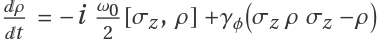with T₂=1/2γ_ϕ and the initial state :

In[4]:=

$\[Rho] = ResourceFunction["LindbladSolve"][ PauliMatrix[ 3], {Sqrt[1/3] PauliMatrix[3]}, {{(1 + rz)/2, 1/2 (rx - I ry)}, {1/2 (rx + I ry), (1 - rz)/2}}, t]; \[Rho] // MatrixForm$

Out[5]=

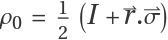Calculate the time-dependent Bloch vector:

In[6]:=

$Table[Tr[\[Rho] . PauliMatrix[j]], {j, 3}] // FullSimplify$

Out[6]=

Solve a single-qubit spontaneous emission (amplitude damping, NMR T₁) where with σ_-={{0,1},{0,0}} and the initial density operator :

In[7]:=

$ClearAll[\[Omega]0, \[Gamma], \[Rho]] ResourceFunction[ "LindbladSolve"][\[Omega]0/ 2 PauliMatrix[3], {Sqrt[\[Gamma]] {{0, 1}, {0, 0}}}, Array[Subscript[\[Rho], ##] &, {2, 2}, 0], t, Assumptions -> \[Gamma] > 0] // FullSimplify // MatrixForm$

Out[8]=

Define a time-dependent Hamiltonian as :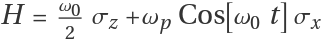

In[9]:=

$ClearAll[h, \[Omega]0, \[Omega]p, tf, \[Gamma], \[Rho], t, lindblad] h = (\[Omega]0/ 2 PauliMatrix[3] + \[Omega]p Cos[\[Omega]0 t] PauliMatrix[1]);$

Set numerical values for Hamiltonian parameters and the final time of simulation:

In[10]:=

$\[Omega]0 = 2 \[Pi] ; \[Omega]p = \[Pi]/10; tf = 2 \[Pi]/\[Omega]p;$

Set the Lindblad operators as {σ_-,σ₊}

In[11]:=

$\[Gamma] = 1/20; lindblad = Sqrt[\[Gamma]] {\!$TraditionalForm\`{{0, 1}, {0, 0}}$, \!$TraditionalForm\`{{0, 0}, {1, 0}}$};$

Solve the Lindblad master equation numerically:

In[12]:=

$\[Rho] = ResourceFunction["LindbladSolve"][h, lindblad, {{1, 0}, {0, 0}}, {t, 0, 2 tf}];$

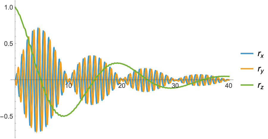
Calculate the Bloch vector and plot its components:

In[13]:=

$Plot[Evaluate@Re@Table[Tr[\[Rho][t] . PauliMatrix[j]], {j, 3}], {t, 0, 2 tf}, PlotRange -> All, PlotLegends -> {"\!$\*SubscriptBox[\(r$, $x$]\)", "\!$\*SubscriptBox[\(r$, $y$]\)", "\!$\*SubscriptBox[\(r$, $z$]\)"}]$

Out[13]=

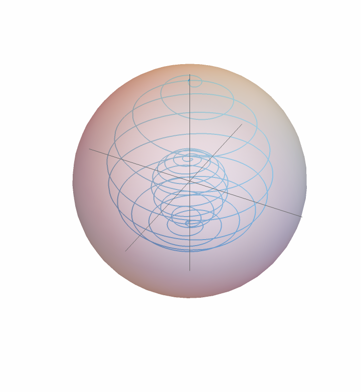
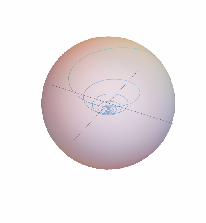
Plot the Bloch vector evolution in the Bloch sphere:

In[14]:=

$Show[Graphics3D[{Opacity[.5], Ball[]}, Boxed -> False, Axes -> True, AxesOrigin -> {0, 0, 0}, Ticks -> None], ParametricPlot3D[ Evaluate@Re@Table[Tr[\[Rho][t] . PauliMatrix[j]], {j, 3}], {t, 0, tf}]]$

Out[14]=

Scope (5)

If no Lindblad operators is given, the solution will be based on only Hamiltonian evolution. Solve the Schrödinger equation for the Hamiltonian 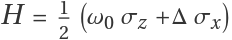starting from the initial pure state {1,0}:

In[15]:=

$ClearAll[\[Omega]0, \[CapitalDelta], t, \[Rho]] $Assumptions = {\[Omega]0 > 0, \[CapitalDelta] > 0}; \[Rho] = FullSimplify /@ ResourceFunction[ "LindbladSolve"][\[Omega]0/2 PauliMatrix[3] + \[CapitalDelta]/ 2 PauliMatrix[1], {}, {1, 0}, t]; \[Rho] // MatrixForm$

Out[16]=

Calculate the time-dependent Bloch vector:

In[17]:=

$Table[Tr[\[Rho] . PauliMatrix[j]], {j, 3}] // FullSimplify$

Out[17]=

Define the Hamiltonian for a Λ-configuration atom (a 3-dimensional atom with the states {,,}):

In[18]:=

$ClearAll[\[CapitalDelta]1, \[CapitalDelta]2, \[Gamma]1, \[Gamma]2] h = {{0, 0, 0}, {0, \[CapitalDelta]1, 0}, {0, 0, \[CapitalDelta]2}};$

Define jump operators as spontaneous emission to the ground state and :

In[19]:=

$lindblad = {Sqrt[\[Gamma]1] {{0, 1, 0}, {0, 0, 0}, {0, 0, 0}}, Sqrt[\[Gamma]2] {{0, 0, 1}, {0, 0, 0}, {0, 0, 0}}};$

Solve the Lindblad equation for an initial state :

In[20]:=

$ResourceFunction["LindbladSolve"][h, lindblad, {0, 1, 1}/Sqrt[2], t, Assumptions -> \[Gamma]1 > 0 && \[Gamma]2 > 0]$

Out[20]=

Define the Hamiltonian for a Λ-configuration atom (a 3-dimensional atom with the states {,,}):

In[21]:=

$ClearAll[\[CapitalOmega]1, \[CapitalOmega]2, \[CapitalDelta]1, \[CapitalDelta]2, \[Gamma]1, \[Gamma]2, \[Gamma]\[Phi]] h = {{0, \[CapitalOmega]1/2, \[CapitalOmega]2/2}, {\[CapitalOmega]1/ 2, \[CapitalDelta]1, 0}, {\[CapitalOmega]2/2, 0, \[CapitalDelta]2}};$

Define jump operator as the differential dephasing that kills the coherence between and :

In[22]:=

$lindblad = {Sqrt[\[Gamma]\[Phi]/2] {{0, 0, 0}, {0, 1, 0}, {0, 0, -1}}};$

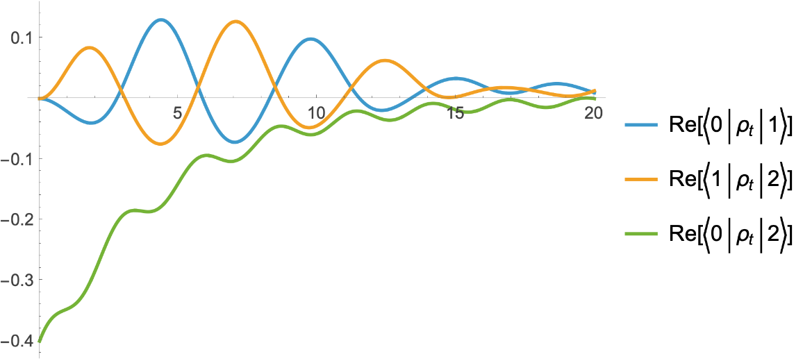
Given some numerical values for parameters, solve the Lindblad equation for an initial state :

In[23]:=

$\[Gamma]1 = \[Gamma]2 = \[Gamma]\[Phi] = .3; \[CapitalOmega]1 = \[CapitalOmega]2 = \[Pi]/ 2; \[CapitalDelta]1 = \[CapitalDelta]2 = \[Pi]/8; tf = 20; r = ResourceFunction["LindbladSolve"][h, lindblad, {0, 1, -2}/Sqrt[5], {t, 0, tf}]$

Out[17]=

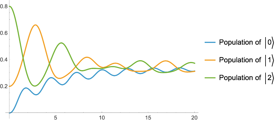
Plot the change in the population:

In[24]:=

$Plot[{Re[r[t][[1, 1]]], Re[r[t][[2, 2]]], Re[r[t][[3, 3]]]}, {t, 0, tf}, PlotRange -> All, PlotLegends -> {"Population of \!$\*TemplateBox[{\"0\"},\n\"Ket\"]$", "Population of \!$\*TemplateBox[{\"1\"},\n\"Ket\"]$", "Population of \!$\*TemplateBox[{\"2\"},\n\"Ket\"]$"}]$

Out[24]=

Plot the coherence between states:

In[25]:=

$Plot[{Re[r[t][[1, 2]]], Re[r[t][[1, 3]]], Re[r[t][[2, 3]]]}, {t, 0, tf}, PlotRange -> All, PlotLegends -> {"Re[\!$\*TemplateBox[{\"0\"},\n\"Bra\"]$\!$\*SubscriptBox[\(\[Rho]$, $t$]\)\!$\*TemplateBox[{\"1\"},\n\"Ket\"]$]", "Re[\!$\*TemplateBox[{\"1\"},\n\"Bra\"]$\!$\*SubscriptBox[\(\[Rho]$, $t$]\)\!$\*TemplateBox[{\"2\"},\n\"Ket\"]$]", "Re[\!$\*TemplateBox[{\"0\"},\n\"Bra\"]$\!$\*SubscriptBox[\(\[Rho]$, $t$]\)\!$\*TemplateBox[{\"2\"},\n\"Ket\"]$]"}]$

Out[25]=

Set the Hamiltonian as :

In[26]:=

$ClearAll[h, \[Gamma], \[Gamma]s, Ls, n, \[CapitalOmega], r] h = \[CapitalOmega]/2 PauliMatrix[3];$

Set the Lindblad operators:

In[27]:=

$\[Gamma]s = \[Gamma] {n + 1, n}; Ls = Sqrt[\[Gamma]s] {{{0, 0}, {1, 0}}, {{0, 1}, {0, 0}}};$

Given some numerical values for parameters, solve the Lindblad equation:

In[28]:=

$\[CapitalOmega] = 50; \[Gamma] = 1; n = 3; r = ResourceFunction["LindbladSolve"][h, Ls, {Cos[\[Pi]/8], Exp[I \[Pi]/4] Sin[\[Pi]/8]}, {t, 0, 1}]$

Out[24]=

Plot results:

In[29]:=

Out[29]=

Model a finite-temperature qubit (generalized amplitude damping), with two jumps:

In[30]:=

$ClearAll[\[Omega]0, \[Gamma]d, \[Gamma]u, r, \[Rho]] $Assumptions = {\[Omega]0 > 0, \[Gamma]d > 0, \[Gamma]u > 0}; Expand@*FullSimplify /@ ResourceFunction[ "LindbladSolve"][\[Omega]0/ 2 PauliMatrix[3], {Sqrt[\[Gamma]d] {{0, 1}, {0, 0}}, Sqrt[\[Gamma]u] {{0, 0}, {1, 0}}}, Array[Subscript[\[Rho], ##] &, {2, 2}, 0], t] // MatrixForm$

Out[27]=

Options (9)

NDSolve or DSolve options (2)

Use Assumptions to assume the jump rate is positive:

In[31]:=

$ClearAll[\[Omega]0, \[Gamma]] ResourceFunction[ "LindbladSolve"][\[Omega]0/ 2 PauliMatrix[3], {Sqrt[\[Gamma]] PauliMatrix[3]}, 1/2 (IdentityMatrix[2] + {rx, ry, rz} . Table[PauliMatrix[j], {j, 3}]), t, Assumptions -> \[Gamma] > 0]$

Out[32]=

Without the above assumption, the rate will be treated in the most generic sense:

In[33]:=

$ResourceFunction[ "LindbladSolve"][\[Omega]0/ 2 PauliMatrix[3], {Sqrt[\[Gamma]] PauliMatrix[3]}, 1/2 (IdentityMatrix[2] + {rx, ry, rz} . Table[PauliMatrix[j], {j, 3}]), t]$

Out[33]=

Method (2)

When the independent variable t is given within the range t_min to t_max, if no Method is given, LindbladSolve gives a numerical result:

In[34]:=

Out[34]=

When the independent variable t is given within the range t_min to t_max, but with the option "Symbolic" for Method, LindbladSolve gives the symbolic result:

In[35]:=

Out[35]=

AdditionalEquations (4)

Using the option "AdditionalEquations", one can add more equations into DEs. Define a pulse given an operator and a rotation angle:

In[36]:=

$ClearAll[pulse]; pulse[\[Theta]_, op_] := MatrixExp[-I \[Theta]/2 op ];$

Define pure dephasing at rate γ plus Larmor precession ω₀σ_z/2:

In[37]:=

$ClearAll[\[Omega]0, \[Gamma], \[Theta], tf, \[Rho]] h = \[Omega]0/2 PauliMatrix[3]; l = {Sqrt[\[Gamma]] PauliMatrix[3]};$

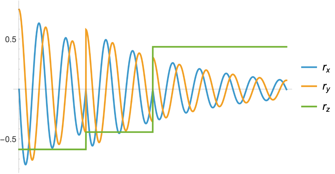
Given some numerical values for parameters, solve the Lindblad equation by adding pulses at selected times (similar to Hahn spin-echo):

In[38]:=

$\[Omega]0 = 2 \[Pi] 5 10^3; tf = 10 2 \[Pi]/\[Omega]0; \[Gamma] = \[Omega]0/50; \[Tau] = tf/4; \[Rho] = ResourceFunction["LindbladSolve"][h, l, {1, 2 I}/Sqrt[5], {t, 0, tf}, "AdditionalEquations" -> {WhenEvent[ t == \[Tau], \[FormalR][t] -> pulse[\[Pi]/2, PauliMatrix[1]] . \[FormalR][t] . pulse[-\[Pi]/2, PauliMatrix[1]]], WhenEvent[ t == 2 \[Tau], \[FormalR][t] -> pulse[\[Pi], PauliMatrix[1]] . \[FormalR][t] . pulse[-\[Pi], PauliMatrix[1]]]}]$

Out[29]=

Plot the evolution of the Bloch vector's components:

In[39]:=

$Plot[Evaluate@Re@Table[Tr[\[Rho][t] . PauliMatrix[j]], {j, 3}], {t, 0, tf}, PlotRange -> All, PlotLegends -> {"\!$\*SubscriptBox[\(r$, $x$]\)", "\!$\*SubscriptBox[\(r$, $y$]\)", "\!$\*SubscriptBox[\(r$, $z$]\)"}, Ticks -> {None, Automatic}]$