Details
A Gaussian beam is an important type of optical beam that closely approximates different types of beams encountered in real life as well as various fields of physics.
ResourceFunction["GaussianBeam"] represents a Gaussian field that propagates along the vertical z-axis and that is parametrized by its beam waist w0 and Rayleigh range zR.
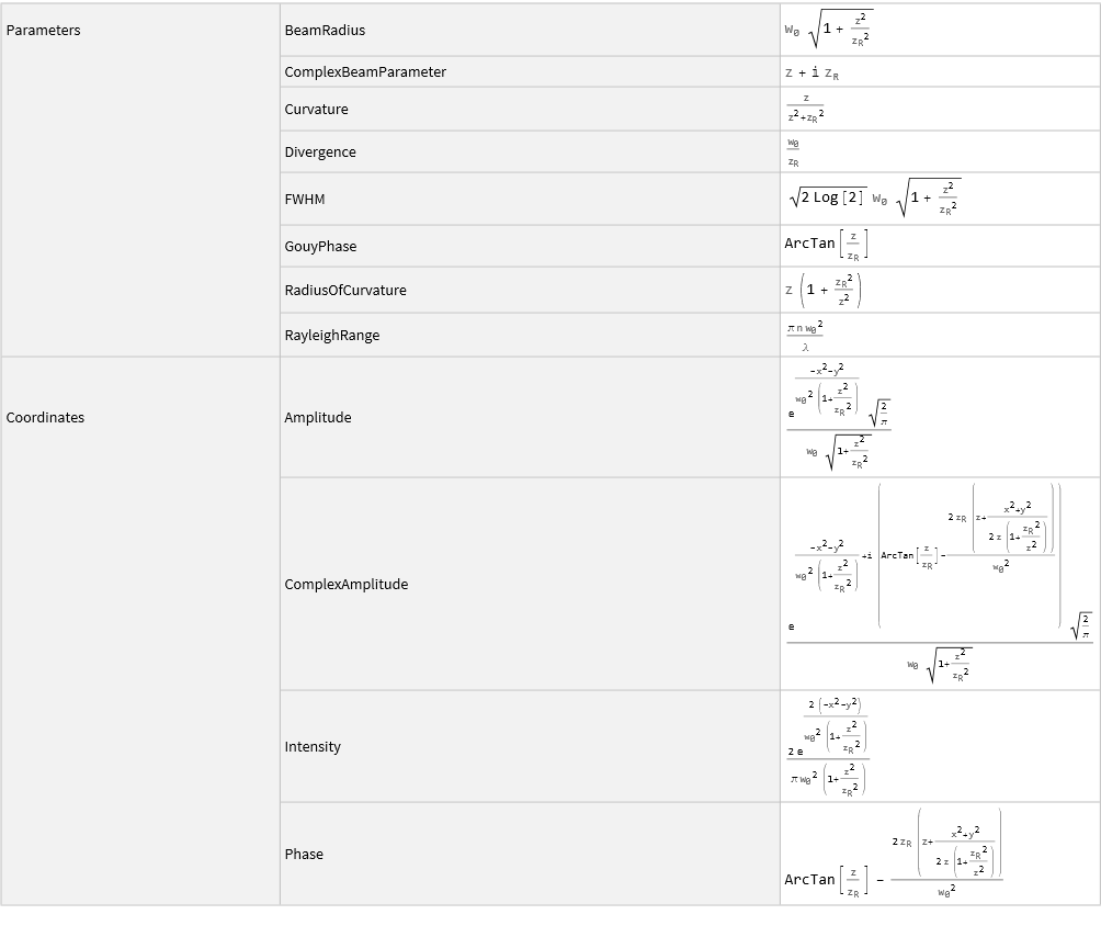
Properties are grouped into "Profiles", "Parameters", and "Summary", which groups one can retrieve by calling ResourceFunction["GaussianBeam"]["Properties"]. All available profiles and computed parameters are listed in ResourceFunction["GaussianBeam"]["Profiles"] and ResourceFunction["GaussianBeam"]["Parameters"], respectively.
Available profiles include:
| "Amplitude" | (real) amplitude of electromagnetic beam |
| "ComplexAmplitude" | (complex) amplitude that includes both the real amplitude and phase |
| "Intensity" | magnitude squared of amplitude |
| "Phase" | phase of electromagnetic beam |
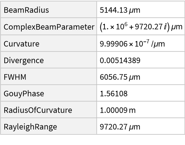
Available computed parameters include:
| "BeamRadius" | beam radius at given longitudinal position |
| "ComplexBeamParameter" | complex beam parameter |
| "Curvature" | beam curvature |
| "Divergence" | beam divergence |
| "FWHM" | full width at half maximum |
| "GouyPhase" | Gouy phase |
| "RadiusOfCurvature" | radius of beam curvature |
| "RayleighRange" | Rayleigh range |
The formula for a given computed parameter par is obtained by calling ResourceFunction["GaussianBeam"][par]. For instance, the explicit formula for the beam divergence is retrieved by calling ResourceFunction["GaussianBeam"]["Divergence"].
Summary of all parameters and profiles is returned by
ResourceFunction["GaussianBeam"]["Summary"] in the form of
Dataset.
Not all beam parameters are independent of each other. The canonical set of independent parameters is the beam waist
w0 and Rayleigh range
zR, out of which all other properties can be calculated. The relation between the two independent parameters reads
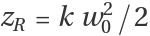
, where
k=2πn/λ is the beam's wavenumber and where further
n is the refractive index of the propagation medium and
λ is the beam's wavelength. Instead of
w0 and
zR one could thus choose any complete set of these characteristics to specify the beam. For that reason, there are several ways of specifying a Gaussian beam:
| {w0,zR} | specific beam waist and Rayleigh range |
| "Normalized" | equivalent to w0=1 and zR=1 |
| <|k1→v1,k2→v2,…|> | Association with a set of independent parameters |
When the parameters are specified as an
Association, the following named keys are supported:
| "BeamWaist" | beam waist |
| "RayleighRange" | Rayleigh range |
| "Wavenumber" | wavenumber k=2πn/λ |
| "Wavelength" | wavelength λ |
| "RefractiveIndex" | refractive index n |
There are also short keys supported for convenience:
| "w0" | beam waist |
| "zR" | Rayleigh range |
| "k" | wavenumber k=2πn/λ |
| "λ" | wavelength λ |
| "n" | refractive index n |
There are two possibilities for an independent set of parameters: either 1) exactly two of w0, zR, and k are given; or 2) exactly one of w0 and zR together with both λ and n are given.
The input parameters can be specified in the following formats:
| v | symbolic variable |
| 0.325 | numeric value |
| Quantity[v,unit] | symbolic or numeric value with unit |
| QuantityVariable[v,unit] | named physical quantity with unit |
Two coordinate systems are supported, which can be specified as the second argument:
| "Cartesian" | Cartesian coordinates {x,y,z} (default) |
| "Cylindrical" | cylindrical coordinates {r,ϕ,z} |
The Gaussian beam formula depends explicitly on several computed parameters such as beam radius and radius of curvature. These are by default automatically expanded into their functional representation. One can suppress this expansion by setting the third argument to
False. This turns the parameters into
QuantityVariable objects and the beam formula is thus returned in its higher-level form. Such a form might be beneficial when rendering the formula in some text or for reference purposes.

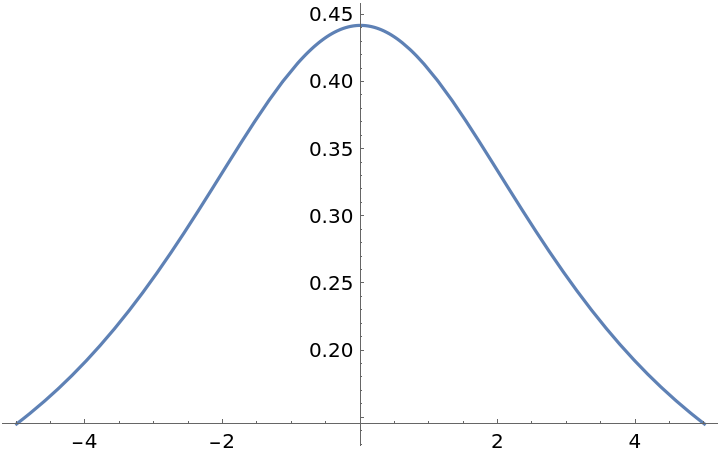
![xint = Table[
ResourceFunction[
"GaussianBeam"][{"Intensity", <|"BeamWaist" -> 0.7, "RayleighRange" -> 0.5|>}][x, 0, 0], {x, -1, 1, 0.1}]](https://www.wolframcloud.com/obj/resourcesystem/images/29e/29efef36-7766-47bc-bbbc-d43ca5f08871/2553e120d24797db.png)

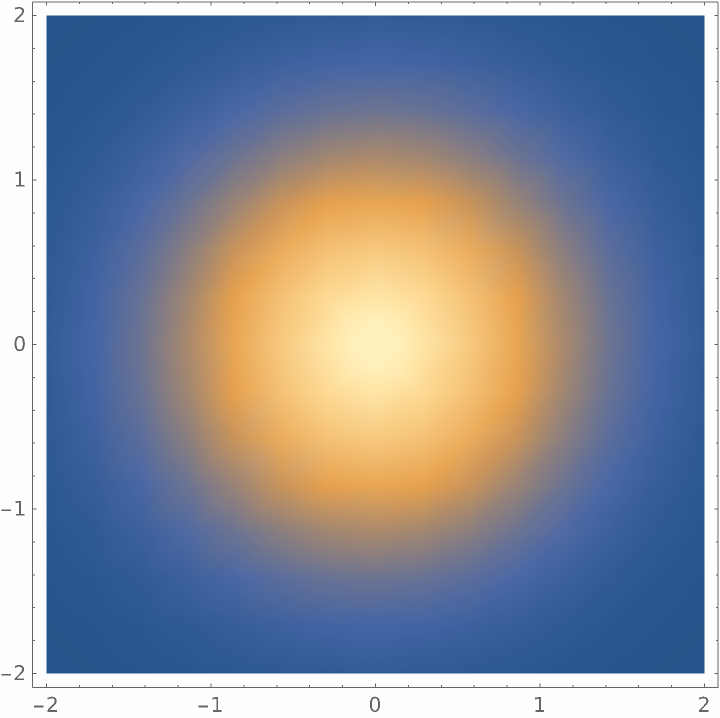
![zpos = 0.5;
beam = ResourceFunction["GaussianBeam"][{"Amplitude", {1, 1}, zpos}];
DensityPlot[beam[x, y], {x, -2, 2}, {y, -2, 2}]](https://www.wolframcloud.com/obj/resourcesystem/images/29e/29efef36-7766-47bc-bbbc-d43ca5f08871/08830bf1877158cf.png)


![{
ResourceFunction["GaussianBeam"]["FWHM"],
ResourceFunction["GaussianBeam"][{"FWHM", {w0, zR}}],
ResourceFunction["GaussianBeam"][{"FWHM", {0.2, 1}}][1.3],
ResourceFunction["GaussianBeam"][{"FWHM", {0.2, 1}, 1.3}],
ResourceFunction[
"GaussianBeam"][{"FWHM", <|"BeamWaist" -> 0.2, "RayleighRange" -> 1|>,
1.3}]
}](https://www.wolframcloud.com/obj/resourcesystem/images/29e/29efef36-7766-47bc-bbbc-d43ca5f08871/04792195e74c68c2.png)
![{
ResourceFunction[
"GaussianBeam"][{"Curvature", QuantityVariable["zR", "Distance"], QuantityVariable["z", "Distance"]}],
ResourceFunction[
"GaussianBeam"][{"Curvature", Quantity[zR, "Millimeters"], Quantity[z, "Millimeters"]}],
ResourceFunction[
"GaussianBeam"][{"Curvature", Quantity[1, "Millimeters"], Quantity[5.0, "Millimeters"]}]
}](https://www.wolframcloud.com/obj/resourcesystem/images/29e/29efef36-7766-47bc-bbbc-d43ca5f08871/5984e033ef3249b0.png)
![{
ResourceFunction["GaussianBeam"][{"BeamRadius", {w0, zR}, z}],
ResourceFunction["GaussianBeam"][{"GouyPhase", zR, z}],
ResourceFunction["GaussianBeam"][{"Divergence", {w0, zR}}]
}](https://www.wolframcloud.com/obj/resourcesystem/images/29e/29efef36-7766-47bc-bbbc-d43ca5f08871/7ef88da79825dc5f.png)
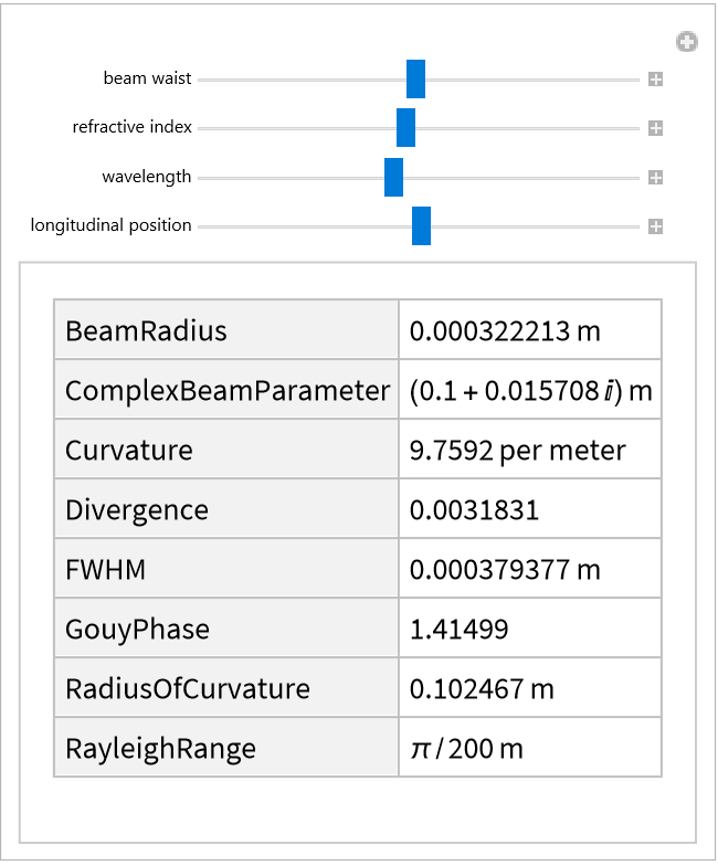
![Manipulate[
UnitConvert@Quiet@ResourceFunction["GaussianBeam"][{"Summary",
Association["w0" -> Quantity[w0val, "Micrometers"], "n" -> nval,
"\[Lambda]" -> Quantity[\[Lambda]val, "Nanometers"]]
, Quantity[zval, "Meters"]}]["Parameters"],
{{w0val, 50, "beam waist"}, 1, 100}, {{nval, 1, "refractive index"}, 0.1, 2},
{{\[Lambda]val, 500, "wavelength"}, 100, 1000}, {{zval, 0.1, "longitudinal position"}, -5, 5}
]](https://www.wolframcloud.com/obj/resourcesystem/images/29e/29efef36-7766-47bc-bbbc-d43ca5f08871/6f279acb079e396f.png)

![intensity = ResourceFunction["GaussianBeam"][{"Intensity", {w0, zR}}][x, y, z];
gaussianDistr2D = PDF[NormalDistribution[0, \[Sigma]]][
x] PDF[NormalDistribution[0, \[Sigma]]][y] /. \[Sigma] -> w0 /2 Sqrt[1 + z^2/zR^2]](https://www.wolframcloud.com/obj/resourcesystem/images/29e/29efef36-7766-47bc-bbbc-d43ca5f08871/0cba8e2f639006b6.png)

![With[{i = ResourceFunction["GaussianBeam"][{"Intensity", {w0, zR}}][x, y, z],
a = ResourceFunction["GaussianBeam"][{"Amplitude", {w0, zR}}][x, y,
z]},
Simplify[i == a^2]
]](https://www.wolframcloud.com/obj/resourcesystem/images/29e/29efef36-7766-47bc-bbbc-d43ca5f08871/44136362caab1233.png)
![With[{ca = ResourceFunction["GaussianBeam"][{"ComplexAmplitude", {w0, zR}}][x,
y, z], a = ResourceFunction["GaussianBeam"][{"Amplitude", {w0, zR}}][x, y, z],
p = ResourceFunction["GaussianBeam"][{"Phase", {w0, zR}}][x, y, z]},
Simplify[ca == a Exp[I p]]
]](https://www.wolframcloud.com/obj/resourcesystem/images/29e/29efef36-7766-47bc-bbbc-d43ca5f08871/5a7993be882c4e1d.png)
![With[{curv = ResourceFunction["GaussianBeam"][{"Curvature", {w0, zR}}][z], rad = ResourceFunction[
"GaussianBeam"][{"RadiusOfCurvature", {w0, zR}}][z]},
Simplify[1/curv == rad]
]](https://www.wolframcloud.com/obj/resourcesystem/images/29e/29efef36-7766-47bc-bbbc-d43ca5f08871/3b079e8908d74f00.png)
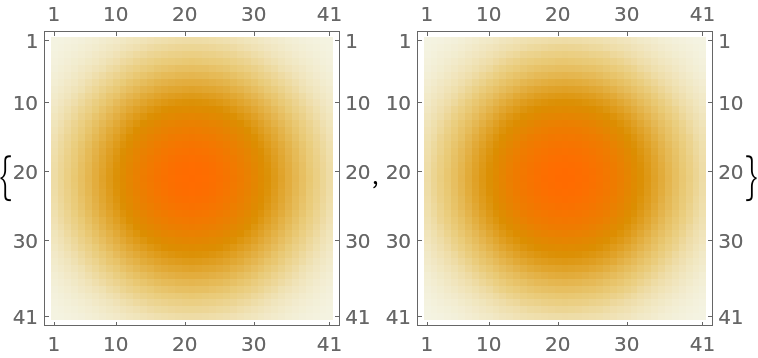
![{time1, mat1} = AbsoluteTiming[GaussianMatrix[20]];
{time2, mat2} = AbsoluteTiming[
Table[ResourceFunction["GaussianBeam"][{"Intensity", {1, 1}, 0}][x,
y], {x, -1, 1, 1/20.}, {y, -1, 1, 1/20.}]];
MatrixPlot /@ {mat1, mat2}](https://www.wolframcloud.com/obj/resourcesystem/images/29e/29efef36-7766-47bc-bbbc-d43ca5f08871/075fabbe6edf3cdb.png)
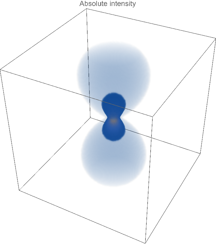
![intensity = ResourceFunction["GaussianBeam"][{"Intensity", "Normalized"}];
DensityPlot3D[
intensity[x, y, z], {x, -15, 15}, {y, -15, 15}, {z, -15, 15}, PlotLabel -> "Absolute intensity", PlotPoints -> 100, Axes -> False]](https://www.wolframcloud.com/obj/resourcesystem/images/29e/29efef36-7766-47bc-bbbc-d43ca5f08871/33e6a5a71aa98339.png)
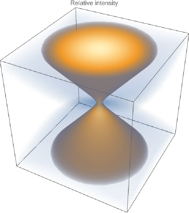
![DensityPlot3D[
intensity[x, y, z]/intensity[0, 0, z], {x, -15, 15}, {y, -15, 15}, {z, -15, 15}, PlotLabel -> "Relative intensity", Axes -> False]](https://www.wolframcloud.com/obj/resourcesystem/images/29e/29efef36-7766-47bc-bbbc-d43ca5f08871/4f37600bf7986090.png)
![{time, wavefronts} = AbsoluteTiming[
ContourPlot3D[
ResourceFunction["GaussianBeam"][{"Phase", {1, 2}}][x, y, z], {x, -4, 4}, {y, -4, 4}, {z, -10, 10}, RegionFunction -> Function[{x, y, z, f}, ResourceFunction["GaussianBeam"][{"BeamRadius", {1, 2}}][z] > Sqrt[x^2 + y^2]], Sequence[
Contours -> Subdivide[-32, 32, 10], ContourStyle -> Directive[
Specularity[20],
Opacity[0.5, Purple]], Mesh -> None, RegionBoundaryStyle -> None]]];
time](https://www.wolframcloud.com/obj/resourcesystem/images/29e/29efef36-7766-47bc-bbbc-d43ca5f08871/48c1ab61975d5027.png)
![volume = ResourceFunction["ExtractGraphicsPrimitives"]@
RevolutionPlot3D[
ResourceFunction["GaussianBeam"][{"BeamRadius", {1.1, 2}}][
z], {z, -8, 8}, Sequence[
RevolutionAxis -> {1, 0, 0}, Mesh -> None, PlotStyle -> Opacity[0.1, Blue], PlotPoints -> 20]];
Show[Graphics3D[{Rotate[
volume, \[Pi]/2, {0, 1, 0}]}], wavefronts, Sequence[
ViewPoint -> {1.75, 0.31, 0.9}, ViewVertical -> {0, 1, 0}, ImageSize -> 800, Boxed -> False, PlotRange -> {5 {-1, 1}, 5 {-1, 1}, 10 {-1, 1}}]]](https://www.wolframcloud.com/obj/resourcesystem/images/29e/29efef36-7766-47bc-bbbc-d43ca5f08871/6b3d211a1b830f76.png)
