Details
Given a triangle A1A2A3, the specified contact point within the segment of A2A3 (opposite to A1) is A2+λ1·(A3-A2) with 0<λ1<1. The same rule applies for λ2 and λ3.
For numerical stability, the accepted range of the affine parameters is 0.02<=λi<=0.98 for i=1,2,3.
The function returns an
Association for each exparabola.
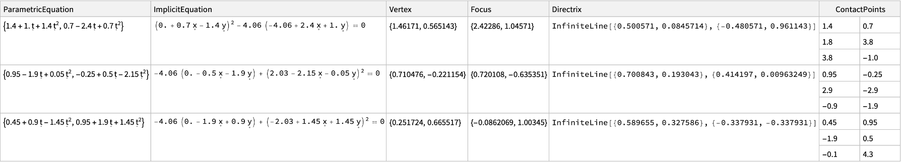
Each exparabola contains the following entries:
| "ImplicitEquation" | The implicit equation for the parabola in terms of x and y |
| "ParametricEquation" | The parametric equation for the parabola in terms of t |
| "Focus" | The focus point of the contact parabola |
| "Vertex" | The vertex point of the contact parabola |
| "Directrix" | The directrix expressed as an InfiniteLine object |
| "ContactPoints" | The three contact points on the parabola |
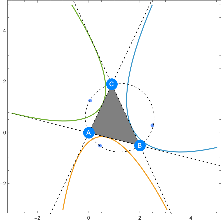
The foci of these contact parabolas are on the circumcircle of the reference triangle. This is the result of the geometric property of
Simson line.
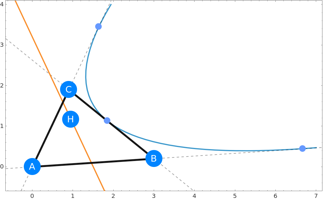
The directrixes of these contact parabolas are through the
orthocenter of the reference triangle.
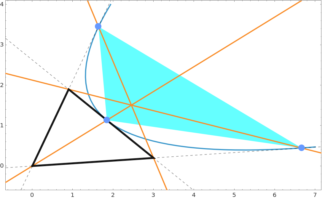
A surprisingly elegant fact is that the parabolas determined by the foci and directrix above always tangent to the three sides of the reference triangle: one contact point is on one side and the other two are on the extension line of the other two sides.
Given a triangle A1A2A3, the returned parabolas are ordered such that the parabola with the internal contact point on the opposite side of A1 comes first, that of A2 comes the second and that of A3 comes the last.
ResourceFunction["Exparabolas"][{
p1,
p2,
p3}, …] is equivalent to ResourceFunction["Exparabolas"][
Triangle[{
p1,
p2,
p3}], …].

![tri = {{0, 0}, {2, -0.5}, {0.9, 1.9}};
parabs = ResourceFunction["Exparabolas"][tri, .6, .6, .4];
eqns = #["ImplicitEquation"] & /@ parabs;](https://www.wolframcloud.com/obj/resourcesystem/images/204/204bd099-51ae-40a6-9492-6be3e4774293/0e73050d67748049.png)
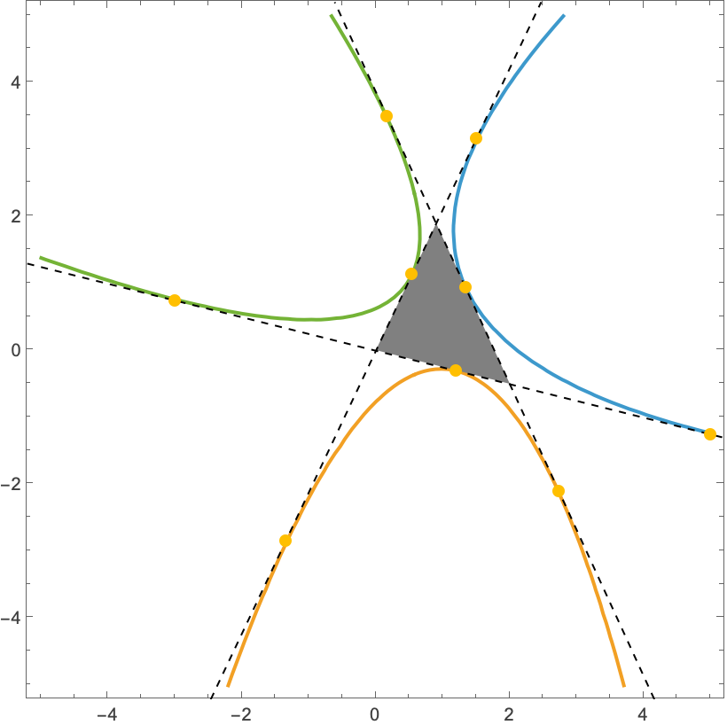
![ContourPlot[
eqns, {\[FormalX], -5, 5}, {\[FormalY], -5, 5}, Epilog -> {
{Gray, Triangle[tri]},
{Dashed, InfiniteLine[tri[[#]]] & /@ {{1, 2}, {2, 3}, {3, 1}}},
{StandardYellow, PointSize[Large], Point /@ (#["ContactPoints"] & /@ parabs)}
}
]](https://www.wolframcloud.com/obj/resourcesystem/images/204/204bd099-51ae-40a6-9492-6be3e4774293/7fd792789268fd1e.png)
![tri = {{0, 0}, {2, -0.5}, {0.9, 1.9}};
parabs = ResourceFunction["Exparabolas"][tri, .6, .6, .4];
Column[paraEqn = #["ParametricEquation"] & /@ parabs]](https://www.wolframcloud.com/obj/resourcesystem/images/204/204bd099-51ae-40a6-9492-6be3e4774293/5bf675ce4dba8ef7.png)

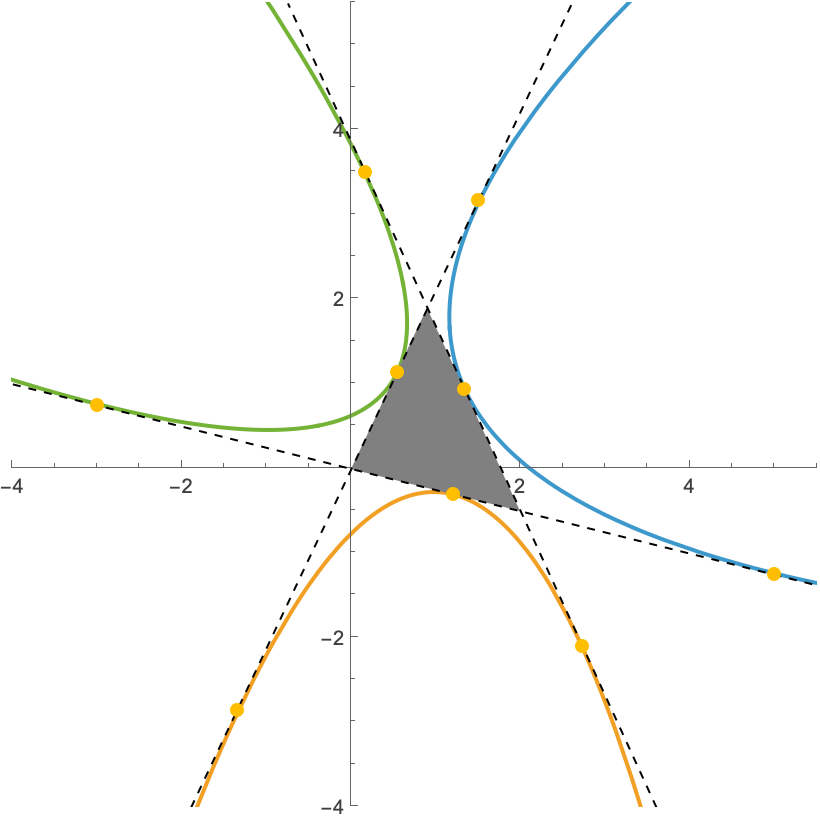
![ParametricPlot[
paraEqn, {\[FormalT], -10, 10}, PlotRange -> {{-4, 5.5}, {-4, 5.5}}, Epilog -> {
{Gray, Triangle[tri]},
{Dashed, InfiniteLine[tri[[#]]] & /@ {{1, 2}, {2, 3}, {3, 1}}},
{StandardYellow, PointSize[Large], Point /@ (#["ContactPoints"] & /@ parabs)}
}]](https://www.wolframcloud.com/obj/resourcesystem/images/204/204bd099-51ae-40a6-9492-6be3e4774293/2f7da31a16d35c23.png)
![tri = {{0, 0}, {2, -0.5}, {0.9, 1.9}};
parabs = ResourceFunction["Exparabolas"][tri, .3, .35, .4];
eqns = #["ImplicitEquation"] & /@ parabs;
foc = #["Focus"] & /@ parabs;](https://www.wolframcloud.com/obj/resourcesystem/images/204/204bd099-51ae-40a6-9492-6be3e4774293/13466f19442716a9.png)
![ContourPlot[
eqns, {\[FormalX], -3, 5}, {\[FormalY], -3, 5}, Epilog -> {
{Gray, Triangle[tri]}, {StandardBlue, PointSize[0.016], Point[foc]},
{Dashed, InfiniteLine[tri[[#]]] & /@ {{1, 2}, {2, 3}, {3, 1}}},
{Dashed, Thickness[0.002], TriangleConstruct[tri, "Circumcircle"]},
MapThread[label[#1, Point@#2] &, {{"A", "B", "C"}, tri}]
}
]](https://www.wolframcloud.com/obj/resourcesystem/images/204/204bd099-51ae-40a6-9492-6be3e4774293/72fcce253e3e5cf3.png)
![tri = {{0, 0}, {3, .2}, {0.9, 1.9}};
parabs = ResourceFunction["Exparabolas"][tri, .55, .2, .3];
eqn = (#["ImplicitEquation"] & /@ parabs)[[1]];
ctnts = (#["ContactPoints"] & /@ parabs)[[1]];](https://www.wolframcloud.com/obj/resourcesystem/images/204/204bd099-51ae-40a6-9492-6be3e4774293/63750176c18023f2.png)
![ContourPlot[
eqn, {\[FormalX], -.5, 7}, {\[FormalY], -.5, 4},
Epilog -> {
{Opacity[0.6], Cyan, Triangle[ctnts]},
{Opacity[0.4], Dashed, InfiniteLine[tri[[#]]] & /@ {{1, 2}, {2, 3}, {3, 1}}},
{StandardOrange, Thick, MapThread[InfiniteLine[{#1, #2}] &, {tri, ctnts}]},
{Transparent, EdgeForm[{Opacity[0.9], Thickness[0.006]}], Triangle[tri]},
{StandardBlue, PointSize[0.02], Point@ctnts}
}, AspectRatio -> 4.5/7.5
]](https://www.wolframcloud.com/obj/resourcesystem/images/204/204bd099-51ae-40a6-9492-6be3e4774293/5686d3b6a275d7fc.png)
![tri = {{0, 0}, {3, .2}, {0.9, 1.9}};
parabs = ResourceFunction["Exparabolas"][tri, .55, .2, .3];
eqn = (#["ImplicitEquation"] & /@ parabs)[[1]];
ctnts = (#["ContactPoints"] & /@ parabs)[[1]];
dir = (#["Directrix"] & /@ parabs)[[1]];](https://www.wolframcloud.com/obj/resourcesystem/images/204/204bd099-51ae-40a6-9492-6be3e4774293/672abbc3791a7487.png)
![ContourPlot[
eqn, {\[FormalX], -.5, 7}, {\[FormalY], -.5, 4},
Epilog -> {
{Opacity[0.4], Dashed, InfiniteLine[tri[[#]]] & /@ {{1, 2}, {2, 3}, {3, 1}}},
{StandardOrange, Thick, dir},
{Transparent, EdgeForm[{Opacity[0.9], Thickness[0.006]}], Triangle[tri]},
MapThread[label[#1, Point@#2] &, {{"A", "B", "C"}, tri}],
label["H", TriangleConstruct[tri, "Orthocenter"]],
{StandardBlue, PointSize[0.02], Point@ctnts}
}, AspectRatio -> 4.5/7.5
]](https://www.wolframcloud.com/obj/resourcesystem/images/204/204bd099-51ae-40a6-9492-6be3e4774293/3d82e38cdbb41883.png)
![tri = {{0, 0.3}, {2, -0.5`}, {0.9, 1.9}};
Manipulate[
parabs = ResourceFunction["Exparabolas"][tri, .4, \[Mu]1, \[Mu]2];
cts = Flatten[Rest /@ (#["ContactPoints"] & /@ parabs), 1];
eqns = #["ImplicitEquation"] & /@ parabs;
ContourPlot[
Evaluate[
Append[eqns, Chop[ResourceFunction["FivePointConic"][cts[[;; 5]]]] == 0]]
, {\[FormalX], -6, 7}, {\[FormalY], -6, 7}, ContourStyle -> Thickness[0.008], Epilog -> {
{Opacity[0.4], Dashed, InfiniteLine[tri[[#]]] & /@ {{1, 2}, {2, 3}, {3, 1}}},
{Opacity[0.4], EdgeForm[{Thickness[0.004]}], Triangle[tri]},
{StandardBlue, PointSize[0.03], Point[cts]}
}, ImageSize -> 460], {\[Mu]1, 0.2, 0.8}, {\[Mu]2, 0.2, 0.8}, TrackedSymbols :> {\[Mu]1, \[Mu]2}]](https://www.wolframcloud.com/obj/resourcesystem/images/204/204bd099-51ae-40a6-9492-6be3e4774293/0d8cd88459d6250c.png)
![(* Evaluate this cell to get the example input *) CloudGet["https://www.wolframcloud.com/obj/6fd0d20a-e8a5-444a-be02-2a612a4b586d"]](https://www.wolframcloud.com/obj/resourcesystem/images/204/204bd099-51ae-40a6-9492-6be3e4774293/5958fc0f58853b29.png)
![tri = {{0, 0.3}, {2, -0.5`}, {0.9, 1.9}};
Manipulate[
parabs = ResourceFunction["Exparabolas"][tri, \[Lambda], \[Mu], .4];
eqns = #["ImplicitEquation"] & /@ parabs;
cts = Flatten[Rest /@ (#["ContactPoints"] & /@ parabs), 1];
foc = #["Focus"] & /@ parabs;
cubic = ResourceFunction["NinePointCubic"][pt, {\[FormalX], \[FormalY]}];
eqns = Append[eqns, cubic == 0];
pt = cts~Join~foc;
ContourPlot[
eqns, {\[FormalX], -4, 6}, {\[FormalY], -4, 6}, PlotPoints -> 60, ImageSize -> 500, ContourStyle -> {
Directive[Opacity[0.6], StandardOrange],
Directive[Opacity[0.6], StandardOrange],
Directive[Opacity[0.6], StandardOrange],
Directive[Thick, StandardBlue]}, Epilog -> {
{Opacity[0.4], Dashed, InfiniteLine[tri[[#]]] & /@ {{1, 2}, {2, 3}, {3, 1}}},
{Opacity[0.4], EdgeForm[{Thickness[0.004]}], Triangle[tri]},
{Directive[AbsolutePointSize[8], RGBColor[0.922526, 0.385626, 0.209179]], Point[pt]}
}], {\[Lambda], 0.1, 0.9}, {\[Mu], 0.1, 0.9}, TrackedSymbols :> {\[Lambda], \[Mu]}]](https://www.wolframcloud.com/obj/resourcesystem/images/204/204bd099-51ae-40a6-9492-6be3e4774293/58150881bf017e46.png)
![(* Evaluate this cell to get the example input *) CloudGet["https://www.wolframcloud.com/obj/faf58ba6-640c-48fb-9044-c5a720e4c17b"]](https://www.wolframcloud.com/obj/resourcesystem/images/204/204bd099-51ae-40a6-9492-6be3e4774293/47e23c97d597f0be.png)