Wolfram Function Repository
Instant-use add-on functions for the Wolfram Language
Function Repository Resource:
Compute the comoving distance as a closed-form function of redshift using a parabolic expansion model
ResourceFunction["ComovingDistance"][z] gives the comoving distance corresponding to the redshift z using a parabolic expansion model. |
Compute a comoving distance from a redshift:
| In[1]:= |
| Out[1]= |
Compute the comoving distance to the surface of last scattering (in Gpc):
| In[2]:= |
| Out[2]= |
Predict the distance moduli of SN 1997ff (redshift equal to 1.755):
| In[3]:= | ![\[Mu][z_] := 5 Log10[QuantityMagnitude[
UnitConvert[ (1 + z) ResourceFunction["ComovingDistance"][
z]/(10*Quantity[1, "Parsecs"]), "DimensionlessUnit"]]]
\[Mu][1.755]](https://www.wolframcloud.com/obj/resourcesystem/images/18e/18e0c43f-0073-41f9-b43a-d6c1558c9c38/3876cc083d655f6a.png) |
| Out[4]= |
Define a helper function for computing an object's distance modulus μ as a function of redshift z:
| In[5]:= | ![\[Mu][z_?NumericQ] := Module[
{luminousDistance},
luminousDistance = (1 + z) ResourceFunction["ComovingDistance"][z];
5 Log10[
QuantityMagnitude[
UnitConvert[ luminousDistance/(10*Quantity[1, "Parsecs"]), "DimensionlessUnit"]]]
]](https://www.wolframcloud.com/obj/resourcesystem/images/18e/18e0c43f-0073-41f9-b43a-d6c1558c9c38/301f969328031b34.png) |
| Out[6]= |
Create a Hubble diagram of observed distance moduli against the function predictions:
| In[7]:= | ![dataUrl = "https://github.com/PantheonPlusSH0ES/DataRelease/raw/refs/heads/main/Pantheon+_Data/4_DISTANCES_AND_COVAR/Pantheon+SH0ES.dat";
pantheonData = Import[dataUrl, "Table", HeaderLines -> 1];
pantheonRedshifts = pantheonData[[All, 3]];
pantheonDistanceModuli = pantheonData[[All, 11]];
observedPlot = ListPlot[Transpose[{pantheonRedshifts, pantheonDistanceModuli}], PlotStyle -> {Gray}, PlotMarkers -> {"\[FilledCircle]", Medium}, PlotRange -> All];
predictionLine = ListLinePlot[
Transpose[{pantheonRedshifts, \[Mu] /@ pantheonRedshifts}], PlotStyle -> {Red, Thick}, PlotRange -> All];
Show[{observedPlot, predictionLine}, PlotRange -> {All, All}, Frame -> True, Axes -> False, FrameLabel -> {"Redshift z", "Distance Modulus \[Mu]"}, LabelStyle -> Directive[14]]](https://www.wolframcloud.com/obj/resourcesystem/images/18e/18e0c43f-0073-41f9-b43a-d6c1558c9c38/58abf90d7dda61cf.png) |
| Out[8]= | 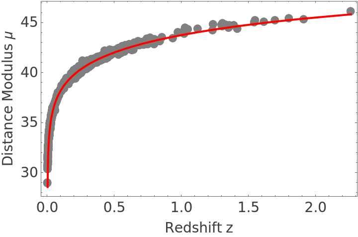 |
ComovingDistance is an approximate inverse for the "Redshift" function in UniverseModelData:
| In[9]:= |
| Out[9]= |
Wolfram Language 13.0 (December 2021) or above
This work is licensed under a Creative Commons Attribution 4.0 International License