Function Repository Resource:

MetropolisHastingsSequence

Source Notebook

Generate a sequence of values using the Metropolis–Hastings Markov chain Monte Carlo method

Contributed by: József Konczer

ResourceFunction["MetropolisHastingsSequence"][f,x,n]

generates n samples using probability function f with independent variable x.

ResourceFunction["MetropolisHastingsSequence"][f,{x,x₀},n]

generates samples using the initial value x₀.

ResourceFunction["MetropolisHastingsSequence"][f,x,{n,burn}]

discards the first burn samples.

ResourceFunction["MetropolisHastingsSequence"][f, x, {n, burn, thin}]

selects n elements in steps of thin.

ResourceFunction["MetropolisHastingsSequence"][f, {{x, x₀},{y, y₀},…}, …]

generates samples for the multivariate function f.

Details and Options

The Metropolis–Hastings algorithm is described on Wikipedia or in this PDF.

ResourceFunction["MetropolisHastingsSequence"] generates a sequence of length n, which has a PDF approximately proportional to f, using the Metropolis–Hastings algorithm starting from initial value x₀, ignoring the first burn samples and selecting every thin^th element.

The default initial value x₀ is zero.

The integer n is the length of the generated list of random variables.

The integer burn is the number of first "thermalization" steps, which do not appear in the output. When burn is not specified, it is zero.

The integer thin is the number of steps completed between two elements in the output list. When thin is not specified, every value is retained.

The usage of burn and thin is consistant with the PyMC package.

ResourceFunction["MetropolisHastingsSequence"] can take the following options:

Method

Automatic

jump function is normally distributed

"Scale"

variance of the normal distribution

"JumpDistribution"

"Normal"

accepts a symmetric parameter‐dependent distribution, if Method→"CustomSymmetricJump"

WorkingPrecision

MachinePrecision

precision used in internal computations

"ShowRejectionRate"

False

controls the appearance of the rejection rate in the output

"LogProbability"

False

f represents a probability function

Supported options for Method are Automatic and "CustomSymmetricJump".

Examples

Basic Examples (3)

Approximate a CauchyDistribution:

In[1]:=

Out[1]=

Approximate a CauchyDistribution using the specified starting point x₀, burn and thin values:

In[2]:=

$ResourceFunction["MetropolisHastingsSequence"][ 1/(1 + x^2), {x, 0}, {10, 0, 1}]$

Out[2]=

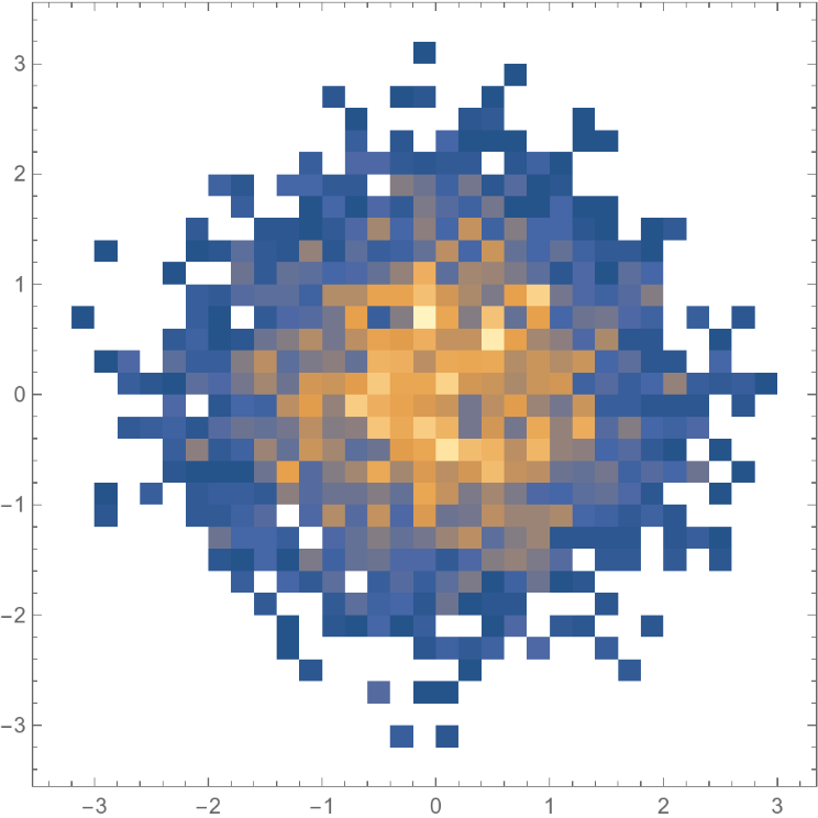
Approximate a MultivariateTDistribution in 2D:

In[3]:=

$ResourceFunction["MetropolisHastingsSequence"][ 1/(1 + x^2 + y^2)^(3/2), {{x, 0}, {y, 0}}, {10, 0, 1}]$

Out[3]=

Options (9)

Method (1)

The default Method is Automatic, in which case the jump function is a NormalDistribution (or MultinormalDistribution):

In[4]:=

$(SeedRandom[1234]; ResourceFunction["MetropolisHastingsSequence"][E^(-x^2/ 2), {x, 0}, {100, 100, 10}, Method -> Automatic]) == (SeedRandom[ 1234]; ResourceFunction["MetropolisHastingsSequence"][E^(-x^2/ 2), {x, 0}, {100, 100, 10}, Method -> "CustomSymmetricJump", "JumpDistribution" -> (NormalDistribution[#, 1] &)])$

Out[4]=

Scale (2)

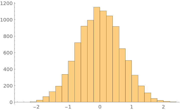
If f has multiple peaks, the algorithm can get stuck in the one nearest to the starting point:

In[5]:=

$ResourceFunction["MetropolisHastingsSequence"][ E^(-(x - 7)^2/2) + E^(-(x + 7)^2/2), {x, 1}, {5000, 100, 10}] // Histogram$

Out[5]=

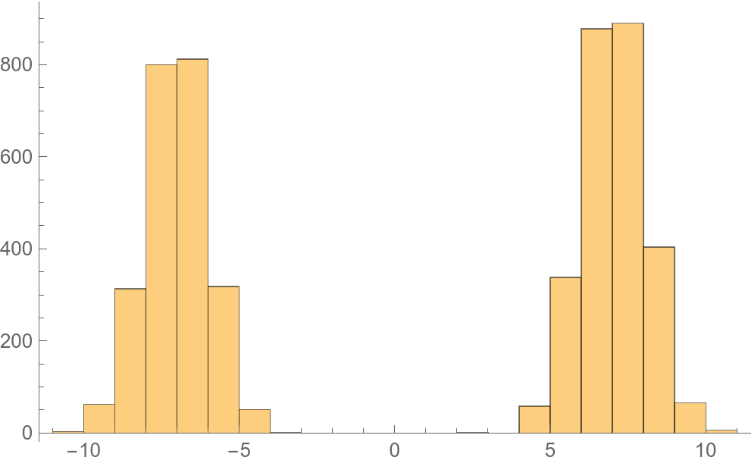
Use a larger "Scale" to explore the whole landscape:

In[6]:=

$ResourceFunction["MetropolisHastingsSequence"][ E^(-(x - 7)^2/2) + E^(-(x + 7)^2/2), {x, 1}, {5000, 100, 10}, "Scale" -> 5] // Histogram$

Out[6]=

JumpDistribution (2)

Use a discrete jump distribution to approximate discrete distributions:

In[7]:=

$f\[ScriptCapitalD][n_] := TransformedDistribution[u - 5 + n, u \[Distributed] BinomialDistribution[10, 1/2]]$

In[8]:=

$f = \[Piecewise] { {1/ x^2, x >= 1}, {0, True} };$

In[9]:=

$ResourceFunction["MetropolisHastingsSequence"][ f, {x, 1}, {1000, 100, 1}, Method -> "CustomSymmetricJump", "JumpDistribution" -> f\[ScriptCapitalD]];$

In[10]:=

Out[10]=

Multivariate example:

In[11]:=

$ResourceFunction["MetropolisHastingsSequence"][ E^(-((x^2 + y^2)/2)), {{x, 0}, {y, 0}}, {5000, 100, 1}, Method -> "CustomSymmetricJump", "JumpDistribution" -> (MultivariateTDistribution[#, IdentityMatrix[2], 3] &)] // DensityHistogram$

Out[11]=

WorkingPrecision (1)

Use WorkingPrecision to get higher precision in parameter estimates:

In[12]:=

$ResourceFunction["MetropolisHastingsSequence"][ 1/(1 + x^2), {x, 0}, {10, 0, 1}, WorkingPrecision -> 20]$

Out[12]=

ShowRejectionRate (2)

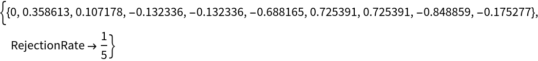
Use "ShowRejectionRate" to see the rejection rate of the process:

In[13]:=

$ResourceFunction["MetropolisHastingsSequence"][ 1/(1 + x^2), {x, 0}, {10, 0, 1}, "ShowRejectionRate" -> True]$

Out[13]=

"ShowRejectionRate" can be used to select an optimal "Scale" for the method ("RejectionRate" is usually advised to be between 50% and 80% [see References]):

In[14]:=

$Table[{\[Sigma], "RejectionRate" /. Last[ResourceFunction["MetropolisHastingsSequence"][ 1/(1 + x^2), {x, 0}, {100, 0, 10}, "ShowRejectionRate" -> True, "Scale" -> \[Sigma]]]}, {\[Sigma], 0.5, 20, 0.5}] // ListPlot$

Out[14]=

LogProbability (1)

Use "LogProbability" to generate samples from a distribution defined by the Log of its PDF:

In[15]:=

Out[15]=

Applications (4)

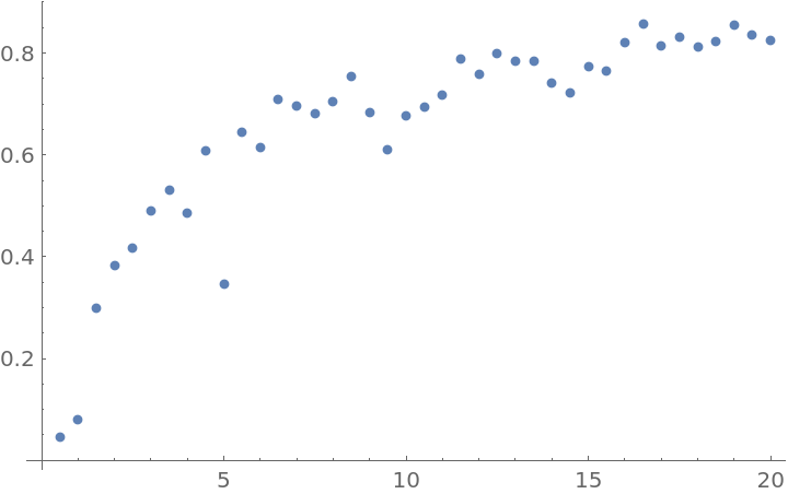
Generate sample data using BernoulliDistribution:

In[16]:=

Define a prior distribution for the parameter (in this case, the Jeffreys prior):

In[17]:=

$Subscript[\[Pi], 0] = \[Piecewise] { {(1/(\[Sqrt]\[Theta] (1 - \[Theta]))), 0 < \[Theta] < 1}, {0, True} };$

Use Bayes's rule and multiply the Likelihood with the prior to get an f function, which is proportional to the posterior distribution of the parameter:

In[18]:=

$f = Likelihood[BernoulliDistribution[\[Theta]], data] Subscript[\[Pi], 0];$

Use MetropolisHastingsSequence to generate one thousand samples of the θ parameter and create a Histogram:

In[19]:=

$Histogram[ ResourceFunction["MetropolisHastingsSequence"][ f, {\[Theta], 1/2}, {1000, 100, 10}], {0, 1, Automatic}, "ProbabilityDensity"]$

Out[19]=

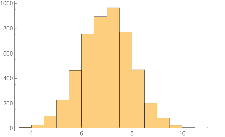
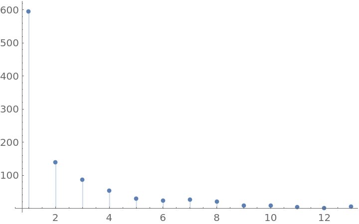
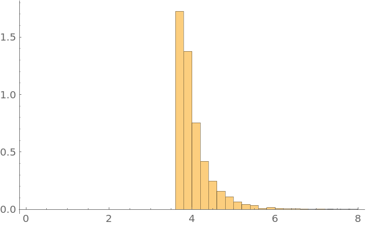
Infer the parameter of a UniformDistribution (also know as the German tank problem). First, generate a small sample of data using UniformDistribution:

In[20]:=

Define a prior distribution for the parameter (in this case, the non-normalizable Jeffreys prior):

In[21]:=

$Subscript[\[Pi], 0] = \[Piecewise] { {1/\[Theta], \[Theta] > 0}, {0, True} };$

Use Bayes's rule and multiply the Likelihood with the prior to get a function that is proportional to the posterior distribution of the parameter:

In[22]:=

$f = Likelihood[UniformDistribution[{0, \[Theta]}], data] Subscript[\[Pi], 0];$

Use MetropolisHastingsSequence to generate one thousand samples of the θ parameter and generate a Histogram:

In[23]:=

$Histogram[ ResourceFunction["MetropolisHastingsSequence"][ f, {\[Theta], 8}, {5000, 100, 10}], {0, 8, Automatic}, "ProbabilityDensity"]$

Out[23]=

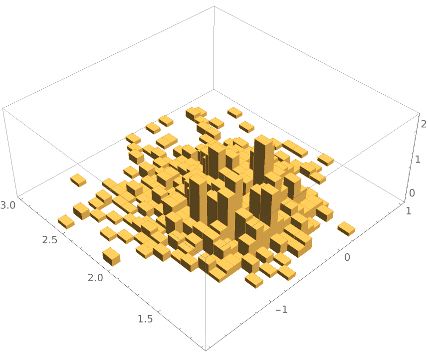
Generate sample data using NormalDistribution:

In[24]:=

Define a prior distribution for the parameter (in this case, the scale-free non-normalizable prior):

In[25]:=

$Subscript[\[Pi], 0] = \[Piecewise] { {1/\[Sigma], \[Sigma] > 0}, {0, True} };$

Use Bayes's rule and multiply the Likelihood with the prior to get a function that is proportional to the posterior distribution of the parameter:

In[26]:=

$f = Likelihood[NormalDistribution[\[Mu], \[Sigma]], data] Subscript[\[Pi], 0];$

Use MetropolisHastingsSequence to generate one thousand samples of the {μ,σ} pair of parameters and generate a Histogram3D:

In[27]:=

$Quiet[Histogram3D[ ResourceFunction["MetropolisHastingsSequence"][ f, {{\[Mu], 0}, {\[Sigma], 1}}, {1000, 100, 10}], {Automatic, {0, 3, Automatic}}, "ProbabilityDensity"]]$

Out[27]=

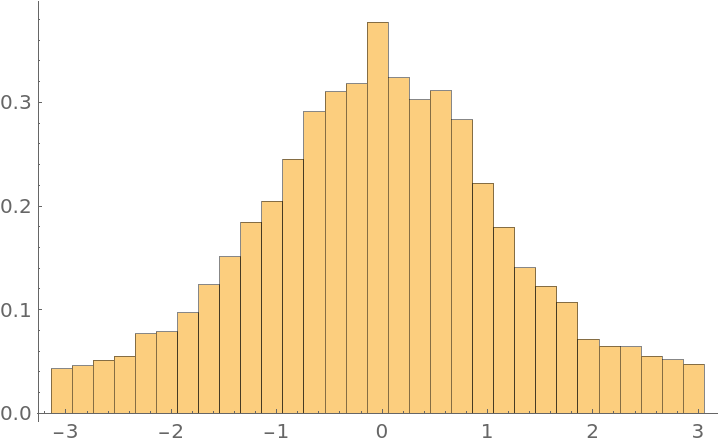
Generating a sample from distribution with PDF defined on a circle:

In[28]:=

$Histogram[ Mod[ResourceFunction["MetropolisHastingsSequence"][ E^-(1 - Cos[\[CurlyPhi]]), {\[CurlyPhi], 0}, {10000, 100, 10}], 2 \[Pi], -\[Pi]], {-\[Pi], \[Pi], Automatic}, "ProbabilityDensity"]$

Out[28]=

Properties and Relations (1)

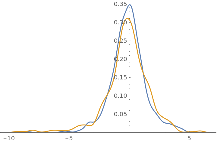
If f is normalized, it approximates RandomVariate[ProbabilityDistribution[f,{x,–∞,∞}],n]:

In[29]:=

$\[ScriptCapitalD] = ProbabilityDistribution[ 1/\[Pi] 1/Cosh[x], {x, -\[Infinity], \[Infinity]}]; data1 = RandomVariate[\[ScriptCapitalD], 500]; data2 = ResourceFunction["MetropolisHastingsSequence"][ 1/Cosh[x], {x, 0}, {500, 100, 10}]; KolmogorovSmirnovTest[data1, data2]$

Out[32]=

In[33]:=

Out[33]=

Possible Issues (2)

The parameter thin should be an integer greater than 0:

In[34]:=

$ResourceFunction["MetropolisHastingsSequence"][ 1/(1 + x^2), {x, \[Pi]}, {10, 0, 0}]$

Out[34]=

The dimension of the parameter-dependent "JumpDistribution" must match the number of variables:

In[35]:=

$ResourceFunction["MetropolisHastingsSequence"][ 1/(1 + x^2 + y^2)^2, {{x, 0}, {y, 0}}, {2, 0, 1}, Method -> "CustomSymmetricJump", "JumpDistribution" -> (NormalDistribution[#, 1] &)]$

Out[35]=

Publisher

Jozsef Konczer

Version History

2.0.0 – 12 February 2021
1.0.0 – 26 October 2020

Source Metadata

Citation:
- Gamerman, D. and H. Lopes. "Markov Chain Monte Carlo: Stochastic Simulation for Bayesian Inference, Second Edition." (2006).
- German, Andrew, John B. Carlin, Hal S. Stern, and Donald B. Rubin. Bayesian Data Analysis, Second Edition. London: Chapman & Hall/CRC, 2003. Print.
- Roberts, G. O.; Gelman, A.; Gilks, W. R. Weak convergence and optimal scaling of random walk Metropolis algorithms. Ann. Appl. Probab. 7 (1997), no. 1, 110--120. doi:10.1214/aoap/1034625254. https://projecteuclid.org/euclid.aoap/1034625254
- Bédard, M. (2008). Optimal acceptance rates for Metropolis algorithms: Moving beyond 0.234. Stochastic Processes and Their Applications, 118(12), 2198–2222. https://doi.org/10.1016/j.spa.2007.12.005

Related Resources

Author Notes

The optimal rejection rate is suggested to be between 50% and 77% (depending on the jump distribution and dimensionality). It works properly only for symmetric jump functions. (Which is not checked during the evaluation) This can be a Method for a more general Markov Chain Monte Carlo (MCMC) function.

License Information

This work is licensed under a Creative Commons Attribution 4.0 International License