Basic Examples (4)
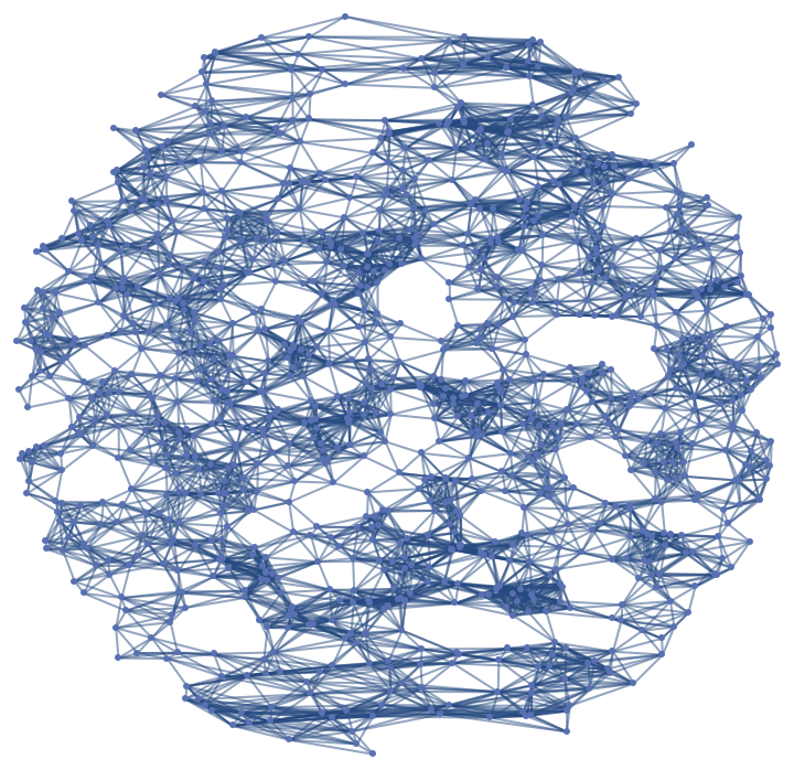
Generate a graph from the volume density of a (piece of a) paraboloid parametrized on a disc of radius 1, with roughly 1000 points, where edges connect points that are sufficiently close:
Generate a graph with the same parameters with vertices on the paraboloid:
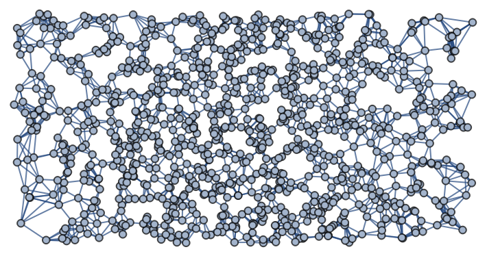
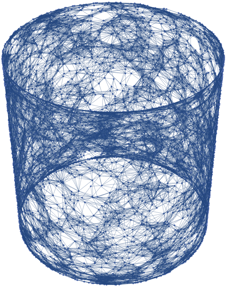
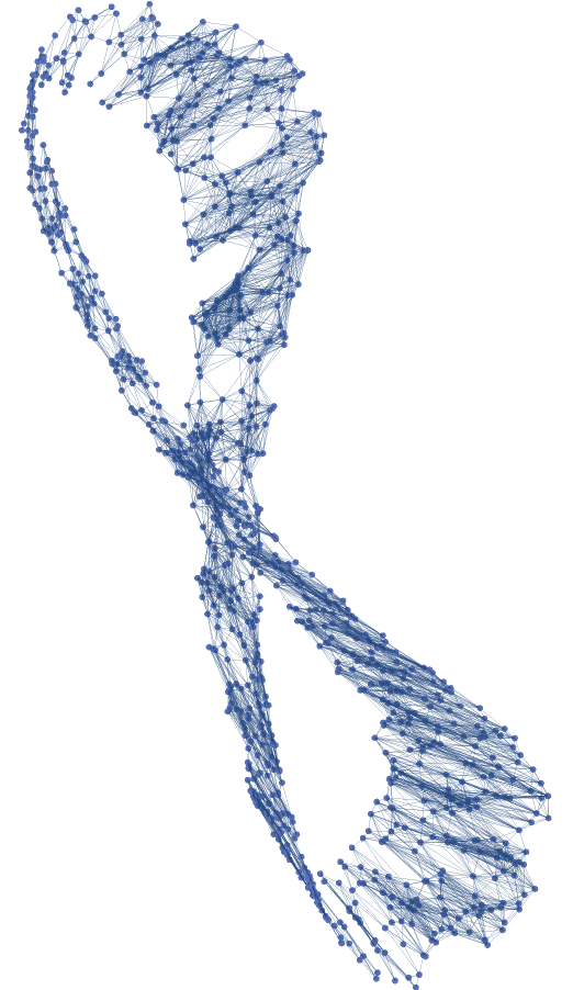
Generate a graph with vertices in ℛ=[-π,π]×[-π/2,π/2], uniformly distributed with respect to the volume density of a torus embedded in  , using the k-nearest neighbors method with k=6 and using the Euclidean distance in the rectangle ℛ:
Compute the minimal, average and maximal length of an edge:
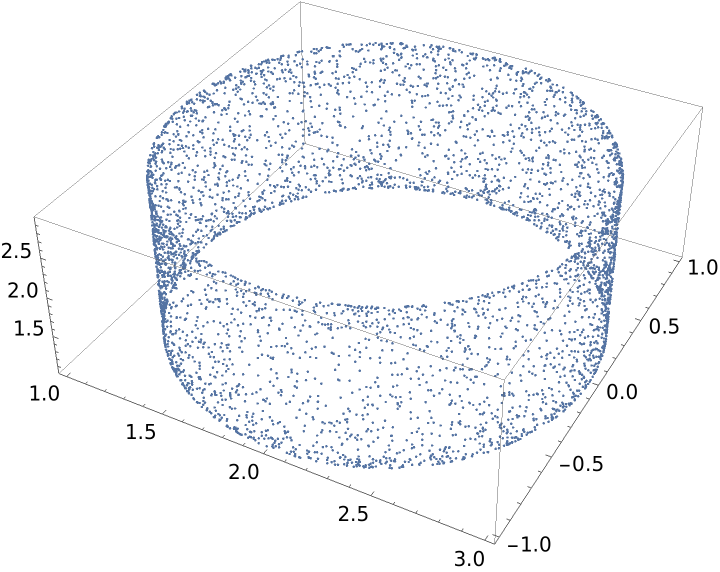
Construct the same graph with vertices in the same region, but taking the distances in , between the images of the points:
The minimal, average and maximal length of an edge in the region as opposed to minimal, average and maximal length of an edge in the target space (where the nearest neighbors algorithm was applied):
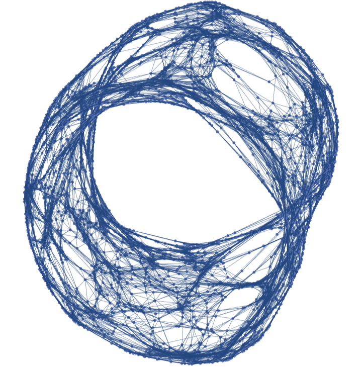
The same graph with vertices in :
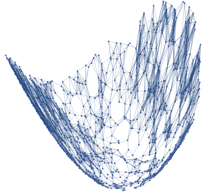
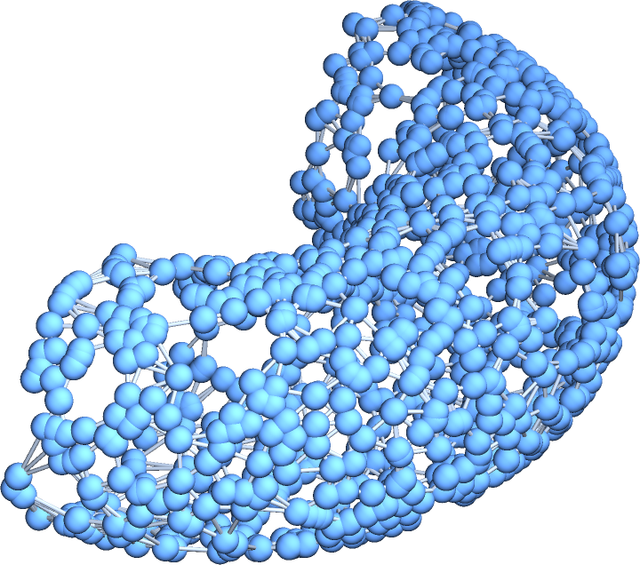
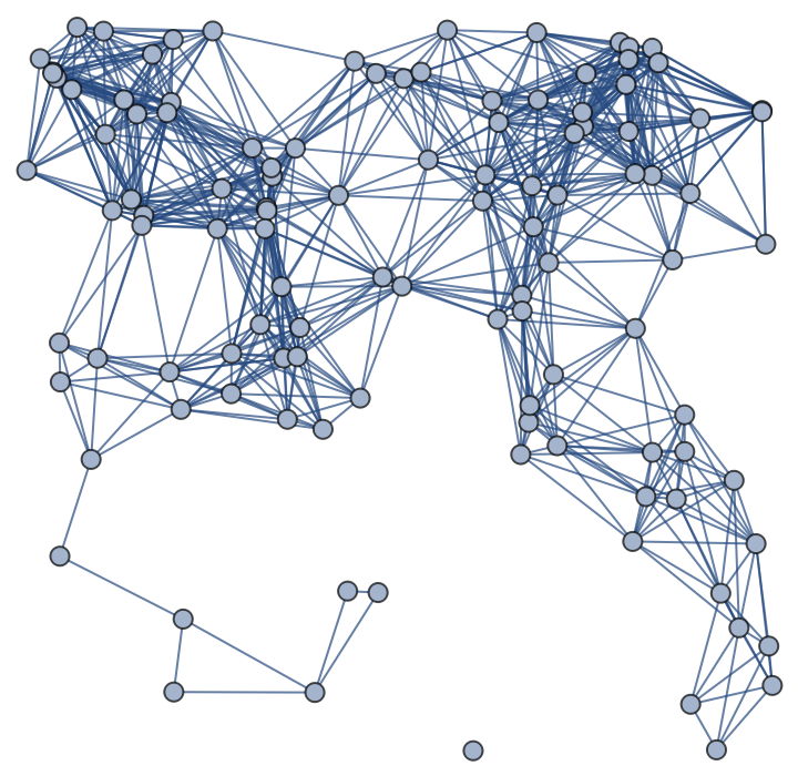
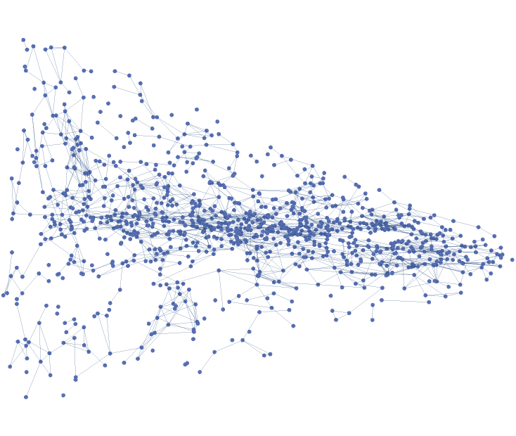
Construct a graph associated with a piece of the pseudosphere, parametrized on [-2,2]×[0,2π], by connecting points with the ϵ-neighbors algorithm with respect to the embedding distance in , with no vertex coordinates:
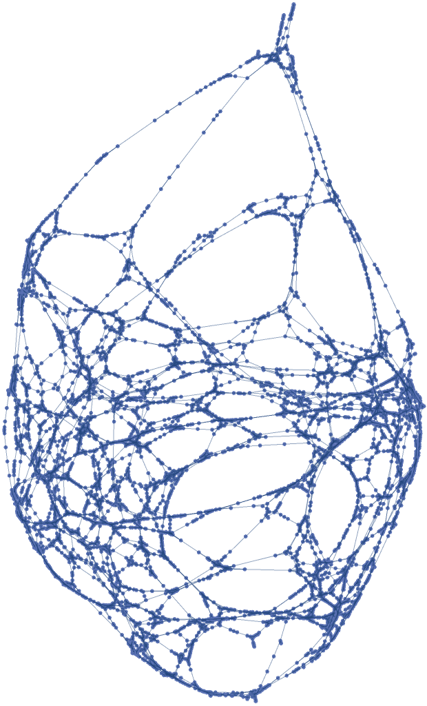
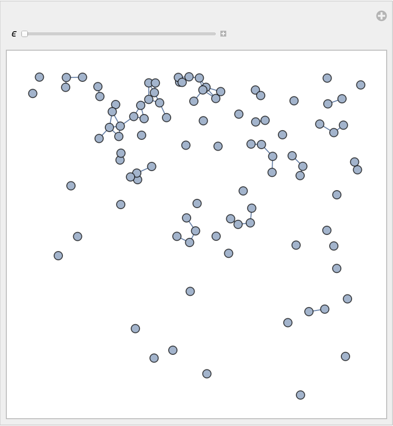
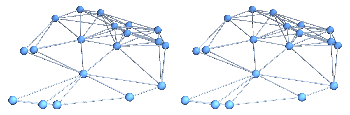
Using GraphPlot or GraphPlot3D with different values for GraphLayout will produce different visualizations of the result:
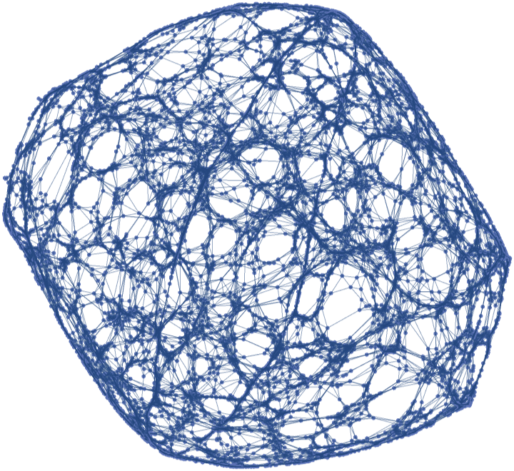
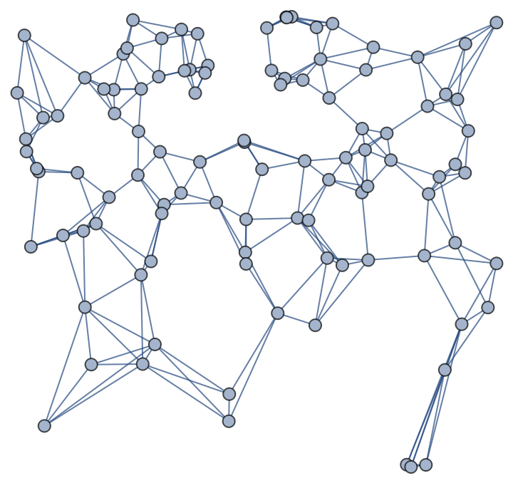
Construct a graph associated with a piece of the pseudosphere, parametrized on [-2,2]×[0,2π], by connecting points with the ϵ-neighbors algorithm with respect to the embedding distance in , using a small ϵ, with no vertex coordinates and only one connected component:
Scope (5)
The graph construction is not limited to surfaces in three-dimensional space:
However, plotting the result might lead to unwanted behaviours, as the vertices are given as points of a four-dimensional space:
In this case the embedding is obtained simply by discarding the fourth coordinate of each vertex:
Using the option None for the "VertexCoordinatesSpace" option will produce a result where no VertexCoordinates specification is given, so GraphPlot3D will automatically find an embedding:
One could also use an explicit setting for GraphLayout:
Options (11)
Distance (4)
The construction of the edges is based on the distances between the vertices. The option "Distance" specifies if it has to be computed in the parameter space, i.e. the region ℛ, or in the embedding space  . When the Jacobian matrix of the parametrization {f1,f2,…} presents huge variations in the eigenvalues or when "distant" points in ℛ end up being "close" in , the results of the two options can be quite different. The "Embedding" setting gives results which follow more closely the geometry of the manifold.
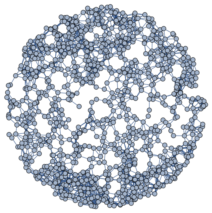
Build a graph given by a parametrization of a slice of a sphere over a disk:
Build the same graph, but with the distance computed in the embedding space (keeping the VertexCoordinates values in the disk to obtain a comparable graphic representation):
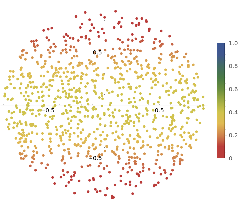
Compare the length of the edges of the planar plot of the result with the distribution of the ratio of the smallest eigenvalue to the largest eigenvalue of the matrix  (where
  the Jacobian matrix of the parametrization), where it can be seen how the points with lower ratio correspond to points in which longer edges are located:
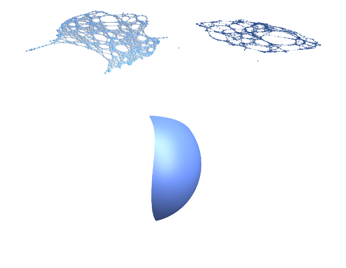
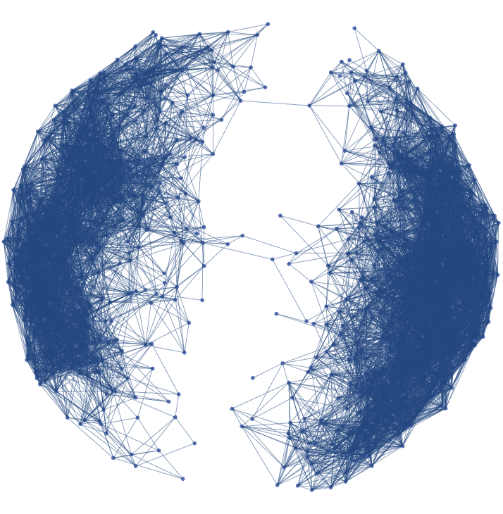
By letting the GraphPlot3D function decide how to represent the two graphs, one can see what difference the choice of the distance function makes on the graph structure (with the original manifold depicted below the graphs):
MaxConnectedComponent (1)
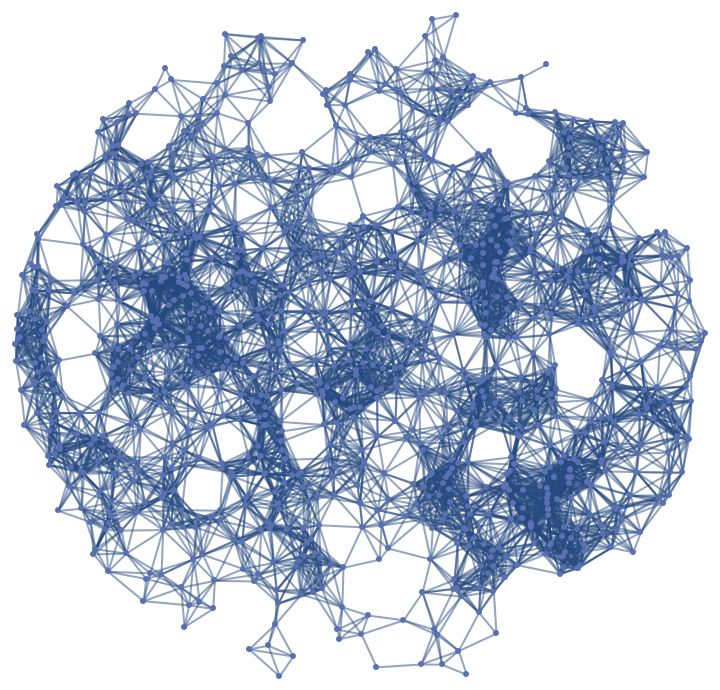
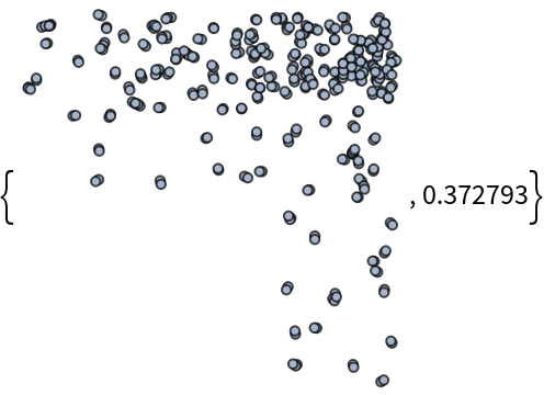
If the "MaxConnectedComponent" option is set to True, the function will return the largest connected component of the resulting graph (or one of them, if there are many) together with the ratio between the number of vertices of such connected component and the total number of generated random points:
As we can see, depending on the other options, the set of vertices of the result can be significantly smaller than the initial set of random points.
Neighbors (2)
Specify the method used to define the neighbors of a vertex. The default value is "Epsilon"; i.e. every point is connected to those which are closer than a given threshold:
The threshold is computed in terms of the number of points and the measure of the parameters region; however, it can be specified in the form "Neighbors"→{"Epsilon",ϵ}:
The value "KNN" means that every point is connected with its k nearest neighbors, with no bounds on the distance, where k depends on the dimension of the region where the distance is computed:
As before, k can be specified as "Neighbors"→{"KNN",k}:
RemoveIsolatedVertices (1)
If the "RemoveIsolatedVertices" option is set to True, the function will delete from the resulting graph all the isolated vertices and return the result together with the ratio between its number of vertices and the total number of generated random points:
When "MaxConnectedComponent" is set to True, the option "RemoveIsolatedVertices" is ignored.
VertexCoordinatesSpace (3)
The option "VertexCoordinatesSpace" is set to Automatic by default, where the first two or three components of the coordinates are used. Depending on the "Distance" option, the vertices will have the coordinates of the points in the parameters space or the coordinates of the points in the embedding space:
The value None will produce a graph without any specification for VertexCoordinates, therefore allowing one to specify an effective GraphLayout setting:
The values "Source" and "Target" will give VertexCoordinates respectively in the source (parameters) region ℛ and in the target (embedding) space of the parametrization , independently of the value given for the "Distance" option:
Applications (2)
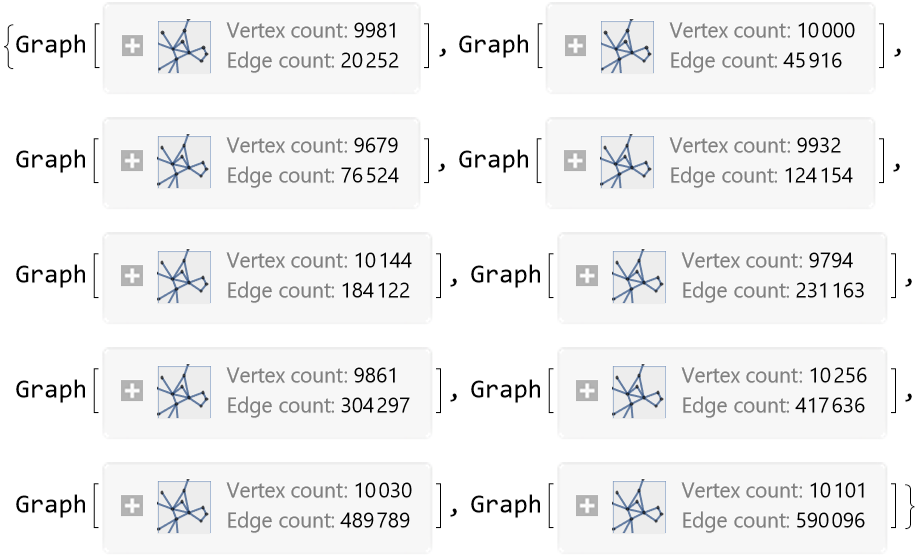
Produce increasingly finer graphs from a given manifold with the nearest neighbors method:
Obtain some basic information about these graphs:
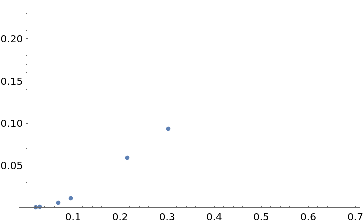
Compute, for each graph, the number of vertices that lie at distance 10 from the point closer to (0,0) over the total number of vertices:
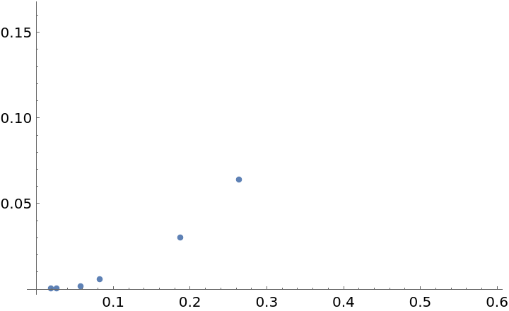
Estimate the radii of these "balls" using the average edge length:
Plot the volume ratios against the estimated radii and try to find a fit:
We now produce graphs from the same manifold, with the same size, but with a different parameter for the KNN algorithm and we repeat the previous computations:
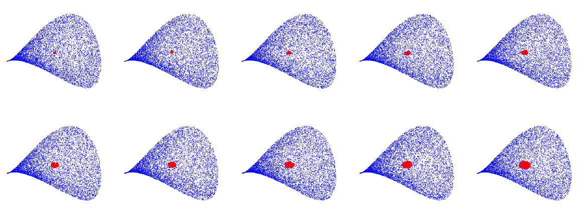
Neat Examples (3)
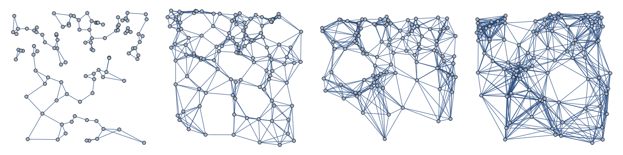
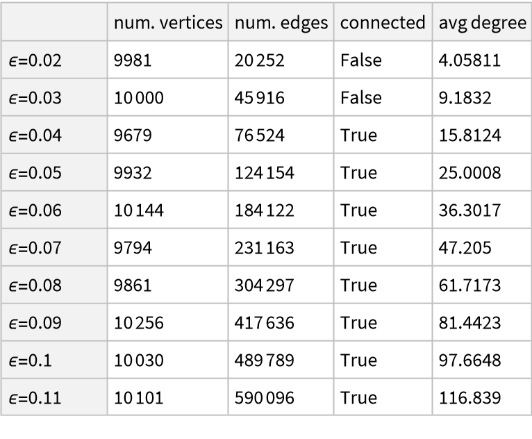
By varying ϵ, with the same parametrization and number of points, one can obtain graphs with an increasing number of edges and average vertex degree:
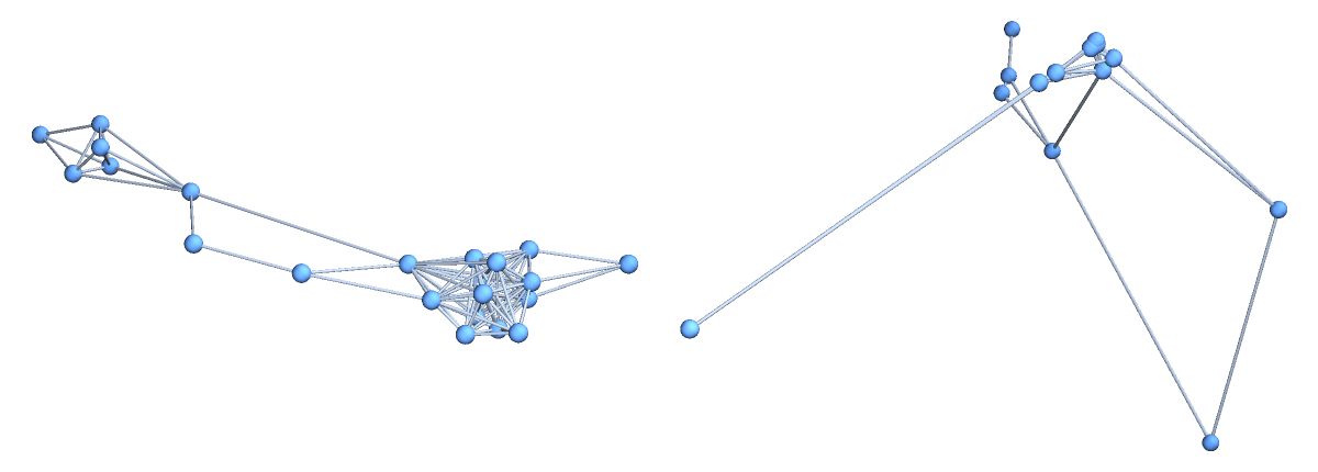
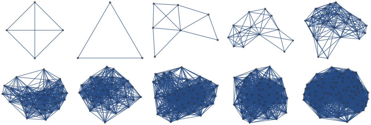
For each graph, find the vertex closest to (0,0) and extract the neighborhood of that vertex (i.e. all the vertices connected to it):
Plot the corresponding points on the manifold:
![graph2 = ResourceFunction[
"ParametricManifoldToGraph"][{Cos[y] (2 + Cos[x]), Sin[y] (2 + Cos[x]), Sin[x]}, {x, -Pi, Pi}, {y, -Pi/2, Pi/2}, 10^3, "Neighbors" -> {"KNN", 6}, "Distance" -> "Embedding", "VertexCoordinatesSpace" -> "Source"]](https://www.wolframcloud.com/obj/resourcesystem/images/175/175aeeb3-2c79-4618-a500-83352006f65c/66554c9d1d1bf8b7.png)
![Through[{Min, Mean, Max}[
Norm[AnnotationValue[{graph2, #[[1]]}, VertexCoordinates] - AnnotationValue[{graph2, #[[2]]}, VertexCoordinates]] & /@ EdgeList[graph2]]]](https://www.wolframcloud.com/obj/resourcesystem/images/175/175aeeb3-2c79-4618-a500-83352006f65c/21b6faf2b79f2336.png)
![pseudosphere = ResourceFunction[
"ParametricManifoldToGraph"][{Sech[u] Cos[v], Sech[u] Sin[v], u - Tanh[u]}, {u, -2, 2}, {v, 0, 2 Pi}, 10^4, "Neighbors" -> {"Epsilon", 0.06}, "Distance" -> "Embedding", "VertexCoordinatesSpace" -> None]](https://www.wolframcloud.com/obj/resourcesystem/images/175/175aeeb3-2c79-4618-a500-83352006f65c/2163369b07055dad.png)
![pseudosphere3 = ResourceFunction[
"ParametricManifoldToGraph"][{Sech[u] Cos[v], Sech[u] Sin[v], u - Tanh[u]}, {u, -2, 2}, {v, 0, 2 Pi}, 10^4, "Neighbors" -> {"Epsilon", 0.045}, "Distance" -> "Embedding", "VertexCoordinatesSpace" -> None, "MaxConnectedComponent" -> True]](https://www.wolframcloud.com/obj/resourcesystem/images/175/175aeeb3-2c79-4618-a500-83352006f65c/00218a25f3024927.png)
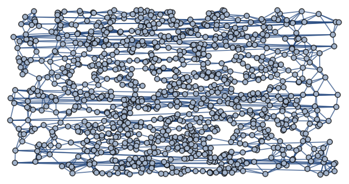
![flatTorus2 = ResourceFunction[
"ParametricManifoldToGraph"][{Cos[u] + 2, Sin[u], Cos[v] + 2, Sin[v]}, {u, -Pi, Pi}, {v, -Pi, Pi}, 5 10^3, "Neighbors" -> {"Epsilon", 0.2}, "Distance" -> "Embedding", "VertexCoordinatesSpace" -> None]](https://www.wolframcloud.com/obj/resourcesystem/images/175/175aeeb3-2c79-4618-a500-83352006f65c/7678814e67ac698d.png)

![slice1 = ResourceFunction[
"ParametricManifoldToGraph"][{Cos[x] Sin[(1 + y) Pi/2], Sin[x] Sin[(1 + y) Pi/2], Cos[(1 + y) Pi/2]}, {x, y}, Disk[{0., 0.}, 0.9], 10^3, "Neighbors" -> {"Epsilon", 0.12}]](https://www.wolframcloud.com/obj/resourcesystem/images/175/175aeeb3-2c79-4618-a500-83352006f65c/4d92420f50dc3b32.png)
![slice2 = ResourceFunction[
"ParametricManifoldToGraph"][{Cos[x] Sin[(1 + y) Pi/2], Sin[x] Sin[(1 + y) Pi/2], Cos[(1 + y) Pi/2]}, {x, y}, Disk[{0., 0.}, 0.9], 10^3, "Neighbors" -> {"Epsilon", 0.12}, "Distance" -> "Embedding", "VertexCoordinatesSpace" -> "Source"]](https://www.wolframcloud.com/obj/resourcesystem/images/175/175aeeb3-2c79-4618-a500-83352006f65c/2322a7bf7a3277d0.png)
![eigv = With[{jac = {D[{Cos[x] Sin[(1 + y) Pi/2], Sin[x] Sin[(1 + y) Pi/2], Cos[(1 + y) Pi/2]}, x], D[{Cos[x] Sin[(1 + y) Pi/2], Sin[x] Sin[(1 + y) Pi/2], Cos[(1 + y) Pi/2]}, y]} . {D[{Cos[x] Sin[(1 + y) Pi/2], Sin[x] Sin[(1 + y) Pi/2], Cos[(1 + y) Pi/2]}, x], D[{Cos[x] Sin[(1 + y) Pi/2], Sin[x] Sin[(1 + y) Pi/2], Cos[(1 + y) Pi/2]}, y]}\[Transpose]}, {AnnotationValue[{slice2, #}, VertexCoordinates], Eigenvalues [
jac /. Thread[{x, y} -> AnnotationValue[{slice2, #}, VertexCoordinates]]]} & /@ VertexList[slice2]];](https://www.wolframcloud.com/obj/resourcesystem/images/175/175aeeb3-2c79-4618-a500-83352006f65c/09b60036433e2e07.png)
![ListPlot[Style[#[[1]], ColorData["DarkRainbow"][1 - Min[#[[2]]]/Max[#[[2]]]], PointSize[Medium]] & /@ eigv, AspectRatio -> 1, PlotLegends -> BarLegend[{ColorData[{"DarkRainbow", "Reverse"}], {0, 1}}]]](https://www.wolframcloud.com/obj/resourcesystem/images/175/175aeeb3-2c79-4618-a500-83352006f65c/19f235d6aab8aefd.png)
![GraphicsColumn[{GraphicsRow[
GraphPlot3D@
ResourceFunction[
"ParametricManifoldToGraph"][{Cos[x] Sin[(1 + y) Pi/2], Sin[x] Sin[(1 + y) Pi/2], Cos[(1 + y) Pi/2]}, {x, y}, Disk[{0., 0.}, 0.9], 10^3, "Neighbors" -> {"Epsilon", 0.1}, "Distance" -> #, "VertexCoordinatesSpace" -> None] & /@ {"Parameters", "Embedding"}, ImageSize -> 800],
ParametricPlot3D[{Cos[x] Sin[(1 + y) Pi/2], Sin[x] Sin[(1 + y) Pi/2], Cos[(1 + y) Pi/2]}, {x, y} \[Element] Disk[{0., 0.}, 0.9], PlotTheme -> "Business", Boxed -> False, Axes -> False]}, ImageSize -> 900]](https://www.wolframcloud.com/obj/resourcesystem/images/175/175aeeb3-2c79-4618-a500-83352006f65c/4e34a7dda493bb7d.png)
![Manipulate[
ResourceFunction[
"ParametricManifoldToGraph"][{x, x y, 2 y^2}, {x, 0, 1}, {y, 0, 1}, 10^2, "Neighbors" -> {"Epsilon", \[Epsilon]}], {\[Epsilon], 0.05, 0.5, 0.05}, SaveDefinitions -> True]](https://www.wolframcloud.com/obj/resourcesystem/images/175/175aeeb3-2c79-4618-a500-83352006f65c/474ecb80670a7144.png)
![mygraphs = ResourceFunction[
"ParametricManifoldToGraph"][{x, x y, 2 y^2}, {x, 0, 1}, {y, 0, 1}, 10^2, "Neighbors" -> {"KNN", #}] & /@ {2, 6, 8, 12};](https://www.wolframcloud.com/obj/resourcesystem/images/175/175aeeb3-2c79-4618-a500-83352006f65c/2dbe9917b6d1a9e2.png)

![(abstractgraph = ResourceFunction[
"ParametricManifoldToGraph"][{x, y - x^2, x + y^2}, {x, y} \[Element] Disk[], 20, "VertexCoordinatesSpace" -> None]) // InputForm](https://www.wolframcloud.com/obj/resourcesystem/images/175/175aeeb3-2c79-4618-a500-83352006f65c/5e79bef9a79910a4.png)

![GraphPlot[
ResourceFunction[
"ParametricManifoldToGraph"][{x^2 + y^2, (x^2 - 1.1)/(y^2 + 1), x + y}, {x, y} \[Element] ImplicitRegion[1 < x^2 + y^2 < 1.5, {x, y}], 10^3, "Neighbors" -> {"Epsilon", 0.1}, "VertexCoordinatesSpace" -> "Target"], VertexSize -> Small]](https://www.wolframcloud.com/obj/resourcesystem/images/175/175aeeb3-2c79-4618-a500-83352006f65c/795009d0374ab4cc.png)
![GraphPlot[
ResourceFunction[
"ParametricManifoldToGraph"][{x^2 + y^2, (x^2 - 1.1)/(y^2 + 1), x + y}, {x, y} \[Element] ImplicitRegion[1 < x^2 + y^2 < 1.5, {x, y}], 10^3, "Neighbors" -> {"Epsilon", 0.1}, "VertexCoordinatesSpace" -> "Source", "Distance" -> "Embedding"], VertexSize -> Small]](https://www.wolframcloud.com/obj/resourcesystem/images/175/175aeeb3-2c79-4618-a500-83352006f65c/0dec47be445f4dd8.png)

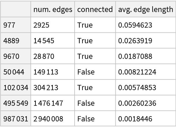
![finergraphs = ResourceFunction[
"ParametricManifoldToGraph"][{u, v, Sqrt[1 - u^2 + v^2]}, {u, -0.9, 0.9}, {v, -1, 1}, #, "Neighbors" -> {"KNN", 7}] & /@ {10^3, 5 10^3, 10^4, 5 10^4, 10^5, 5 10^5, 10^6}; // AbsoluteTiming](https://www.wolframcloud.com/obj/resourcesystem/images/175/175aeeb3-2c79-4618-a500-83352006f65c/0f0e8452ce09d906.png)
![datafg = Association[
VertexCount[#] -> <|"num. edges" -> EdgeCount[#], "connected" -> ConnectedGraphQ[#], "avg. edge length" -> Mean[Norm[#[[1]] - #[[2]]] & /@ EdgeList[#]]|> & /@ finergraphs] // Dataset](https://www.wolframcloud.com/obj/resourcesystem/images/175/175aeeb3-2c79-4618-a500-83352006f65c/1b8c33e4238eb93d.png)

![volumeratios = N@With[{startvertex = Nearest[VertexList[#], {0., 0.}]}, Length@VertexComponent[#, startvertex, 10]/VertexCount[#]] & /@ finergraphs](https://www.wolframcloud.com/obj/resourcesystem/images/175/175aeeb3-2c79-4618-a500-83352006f65c/7fa07bab84243432.png)
![finergraphs2 = ResourceFunction[
"ParametricManifoldToGraph"][{u, v, Sqrt[1 - u^2 + v^2]}, {u, -0.9, 0.9}, {v, -1, 1}, #, "Neighbors" -> {"KNN", 5}] & /@ {10^3, 5 10^3, 10^4, 5 10^4, 10^5, 5 10^5, 10^6}; // AbsoluteTiming](https://www.wolframcloud.com/obj/resourcesystem/images/175/175aeeb3-2c79-4618-a500-83352006f65c/12a1812ad9da8862.png)
![datafg2 = Association[
VertexCount[#] -> <|"num. edges" -> EdgeCount[#], "connected" -> ConnectedGraphQ[#], "avg. edge length" -> Mean[Norm[#[[1]] - #[[2]]] & /@ EdgeList[#]]|> & /@ finergraphs2] // Dataset](https://www.wolframcloud.com/obj/resourcesystem/images/175/175aeeb3-2c79-4618-a500-83352006f65c/4b1a1f1632c8ddc6.png)
![volumeratios2 = N@With[{startvertex = Nearest[VertexList[#], {0., 0.}]}, Length@VertexComponent[#, startvertex, 10]/VertexCount[#]] & /@ finergraphs2](https://www.wolframcloud.com/obj/resourcesystem/images/175/175aeeb3-2c79-4618-a500-83352006f65c/2e46d1b125ab2475.png)
![graphs = ResourceFunction[
"ParametricManifoldToGraph"][{x, y, 1 - x^2 + y^2}, {x, y}, Disk[], 10^4, Neighbors -> {"Epsilon", #}, "VertexCoordinatesSpace" -> None] & /@ Range[0.02, 0.11, 0.01]](https://www.wolframcloud.com/obj/resourcesystem/images/175/175aeeb3-2c79-4618-a500-83352006f65c/4da653483ebffa18.png)
![Association@
MapIndexed[
StringJoin[{"\[Epsilon]=", ToString[#1]}] -> <|
"num. vertices" -> VertexCount[graphs[[First[#2]]]], "num. edges" -> EdgeCount[graphs[[First[#2]]]], "connected" -> ConnectedGraphQ[graphs[[First[#2]]]], "avg degree" -> N@*Mean@VertexDegree[graphs[[First[#2]]]]|> &, Range[0.02, 0.11, 0.01]] // Dataset](https://www.wolframcloud.com/obj/resourcesystem/images/175/175aeeb3-2c79-4618-a500-83352006f65c/0d807790436c2a06.png)
![Partition[
GraphPlot /@ (nghbs = NeighborhoodGraph[#, Nearest[VertexList[#], {0., 0.}]] & /@ graphs), 5] // GraphicsGrid](https://www.wolframcloud.com/obj/resourcesystem/images/175/175aeeb3-2c79-4618-a500-83352006f65c/7695aeea5361d1d6.png)
![GraphicsGrid[
Partition[
MapIndexed[
ListPointPlot3D[{{#1, #2, 1 - #1^2 + #2^2} & @@@ VertexList[#1], {#1, #2, 1 - #1^2 + #2^2} & @@@ VertexList[nghbs[[First[#2]]]]}, PlotStyle -> {Directive[Blue, PointSize[Tiny]], Directive[Red, PointSize[Medium]]}, Axes -> False, Boxed -> False] &, graphs], 5], ImageSize -> 1000]](https://www.wolframcloud.com/obj/resourcesystem/images/175/175aeeb3-2c79-4618-a500-83352006f65c/4ad0160df4c8d932.png)