Wolfram Function Repository
Instant-use add-on functions for the Wolfram Language
Function Repository Resource:
Compute a translation surface parametrization
ResourceFunction["TranslationSurface"][c1,c2,{t,u,v}] computes a translation surface parametrized by u and v from two curves c1 and c2 parametrized by t. |
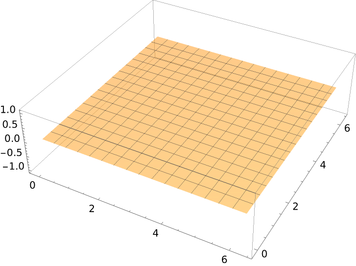
A plane is the translation surface of two intersecting lines:
| In[1]:= |
|
| Out[1]= |
|
Plot it:
| In[2]:= |
|
| Out[2]= |
|
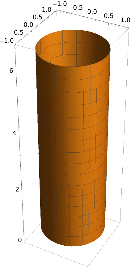
A cylinder is the translation surface of a line translated along a circle:
| In[3]:= |
|
| Out[3]= |
|
Plot it:
| In[4]:= |
|
| Out[4]= |
|
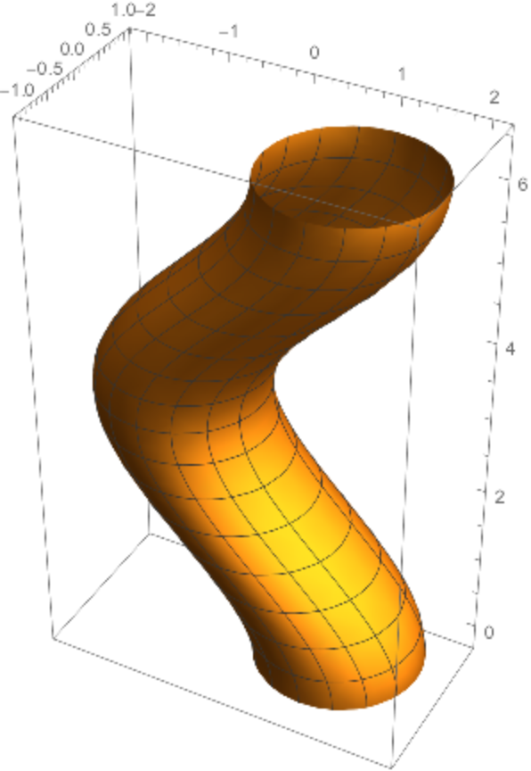
A circle translated along a cosine curve:
| In[5]:= |
|
| Out[5]= |
|
Plot it:
| In[6]:= |
|
| Out[6]= |
|
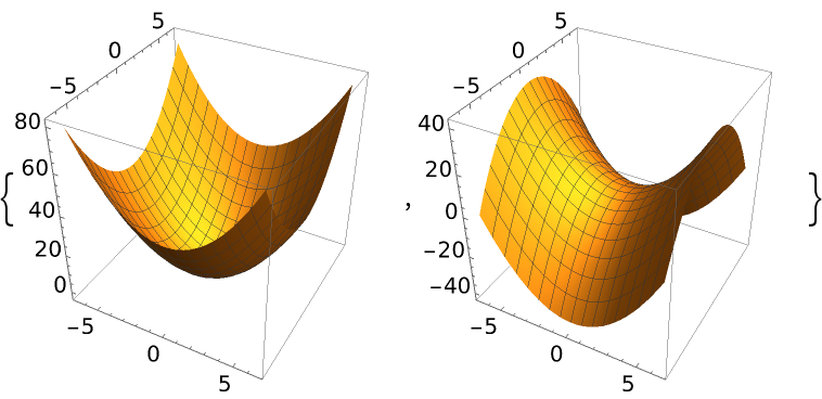
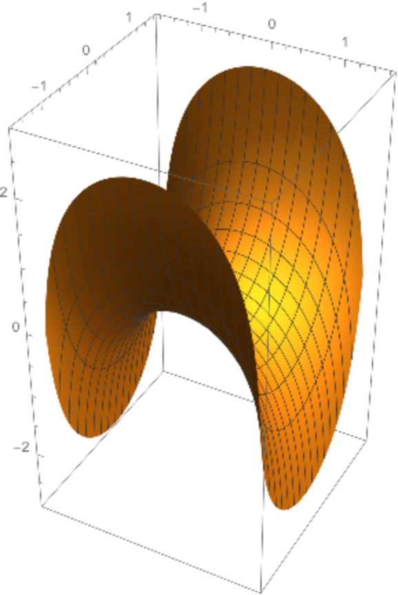
Form elliptic and hyperbolic paraboloids by translating one parabola along another:
| In[7]:= |
![ParametricPlot3D[
ResourceFunction[
"TranslationSurface"][{t, 0, t^2}, {0, t, #}, {t, u, v}], {u, -2 Pi, 2 Pi}, {v, -2 Pi, 2 Pi}, BoxRatios -> {1, 1, 1}] & /@ {t^2, -t^2}](https://www.wolframcloud.com/obj/resourcesystem/images/15c/15c94274-7ca5-403d-a837-136094161702/37144a4c5567c10c.png)
|
| Out[7]= |
|
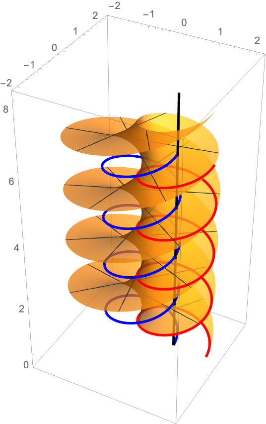
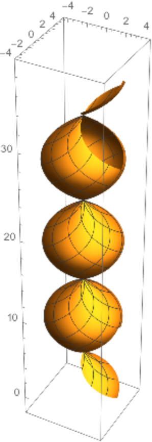
Translate one helix (red) along another helix (blue):
| In[8]:= |
![Show[ParametricPlot3D[
Evaluate[ResourceFunction[
"TranslationSurface"][{Cos[t], Sin[t], t/4}, {Cos[t], Sin[t], t/4}, {t, u, v}]], {u, 0, 2 Pi}, {v, 0, 8 Pi}, MeshFunctions -> {#3 &}, PlotStyle -> Opacity[.5], PlotPoints -> 80], ParametricPlot3D[{{Cos[t], Sin[t], t/4}, {Cos[t] + 1, Sin[t], t/4}}, {t, 0, 8 Pi}, PlotStyle -> {{Thickness[.01], Blue}, {Thickness[.01], Red}}], Graphics3D[{Thickness[.01], Line[{{1, 0, 0}, {1, 0, 8}}]}]]](https://www.wolframcloud.com/obj/resourcesystem/images/15c/15c94274-7ca5-403d-a837-136094161702/7a78418b92c49905.png)
|
| Out[8]= |
|
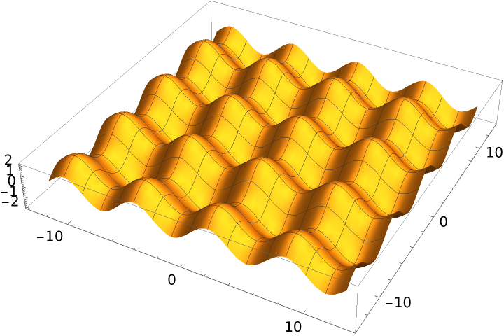
Form an egg box surface by translating one sine along another:
| In[9]:= |
![ParametricPlot3D[
ResourceFunction[
"TranslationSurface"][{t, 0, Sin[t]}, {0, t, Sin[t]}, {t, u, v}], {u, -4 Pi, 4 Pi}, {v, -4 Pi, 4 Pi}]](https://www.wolframcloud.com/obj/resourcesystem/images/15c/15c94274-7ca5-403d-a837-136094161702/51db07e760792f2a.png)
|
| Out[9]= |
|
For the Bohemian dome, the two generatrices are circles:
| In[10]:= |
|
| Out[10]= |
|
| In[11]:= |
![ParametricPlot3D[
ResourceFunction[
"TranslationSurface"][{2 Cos[t], 2 Sin[t], 0}, {0, 3 Cos[t], 3 Sin[t]}, {t, u, v}], {u, 0, 2 Pi}, {v, 0, 2 Pi}]](https://www.wolframcloud.com/obj/resourcesystem/images/15c/15c94274-7ca5-403d-a837-136094161702/514ef0f4be8fe9d1.png)
|
| Out[11]= |
|
A sample surface:
| In[12]:= |
|
| Out[12]= |
|
For the coefficients of the second fundamental form, the second coefficient f is equal to zero for a translation surface:
| In[13]:= |
|
| Out[13]= |
|
A surface generated by a polynomial translated along a parabola:
| In[14]:= |
![ParametricPlot3D[
ResourceFunction[
"TranslationSurface"][{t, 0, (t^2 - 1)^2}, {0, t, -t^2}, {t, u, v}], {u, -1.5, 1.5}, {v, -1.5, 1.5}]](https://www.wolframcloud.com/obj/resourcesystem/images/15c/15c94274-7ca5-403d-a837-136094161702/47815d185a53e1ba.png)
|
| Out[14]= |
|
There is symmetry as when the order of the curves is reversed, the same surface is obtained:
| In[15]:= |
|
| Out[15]= |

|
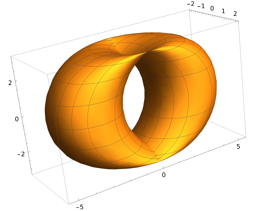
This surface is equivalent to the surface of revolution of the sinusoid:
| In[16]:= |
![ParametricPlot3D[
ResourceFunction[
"TranslationSurface"][{2 Cos[2 t], 2 Sin[2 t], 3 t}, {2 Cos[2 t], -2 Sin[2 t], 3 t}, {t, u, v}], {u, 0, 2 Pi}, {v,
0, 2 Pi}, PlotPoints -> 80, MaxRecursion -> 5]](https://www.wolframcloud.com/obj/resourcesystem/images/15c/15c94274-7ca5-403d-a837-136094161702/10f5fc8e6bc53bd7.png)
|
| Out[16]= |
|
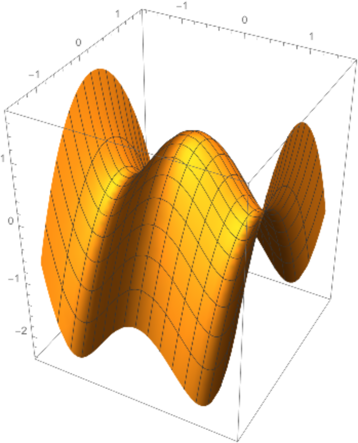
The first Scherk minimal surface:
| In[17]:= |
![ParametricPlot3D[
ResourceFunction[
"TranslationSurface"][{t, 0, Log[Cos[t]]}, {0, t, -Log[Cos[t]]}, {t,
u, v}], {u, -1.5, 1.5}, {v, -1.5, 1.5}, PlotPoints -> 80, MaxRecursion -> 5]](https://www.wolframcloud.com/obj/resourcesystem/images/15c/15c94274-7ca5-403d-a837-136094161702/1809a07353005cdc.png)
|
| Out[17]= |
|
Code to get a curve with prescribed curvature (intrinsic curvature):
| In[18]:= |
![intrinsic[f_, a_, {c_, d_, e_}, {min_, max_}][t_] := Module[{x, y, \[Theta], sol},
eqic = {x'[s] == Cos[\[Theta][s]], y'[s] == Sin[\[Theta][s]], \[Theta]'[s] == f[s], x[a] == c, y[a] == d, \[Theta][a] == e};
sol = NDSolve[eqic, {x, y, \[Theta]}, {s, min, max}];
{x[t], y[t]} /. sol[[1]]
]](https://www.wolframcloud.com/obj/resourcesystem/images/15c/15c94274-7ca5-403d-a837-136094161702/64e1e7d9f91ff4d5.png)
|
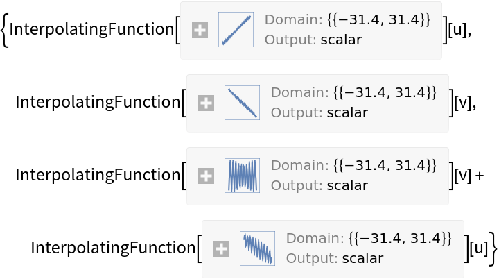
Choose two functions:
| In[19]:= |
![f = intrinsic[3 Sin[#] &, 0, {0, 0, 0}, {-10 \[Pi], 10 \[Pi]}];
g = intrinsic[3 Cos[#] & , 0, {0, 0, 0}, {-10 \[Pi], 10 \[Pi]}];
ResourceFunction["TranslationSurface"][Insert[f[t], 0, 2], Insert[g[t], 0, 1], {t, u, v}]](https://www.wolframcloud.com/obj/resourcesystem/images/15c/15c94274-7ca5-403d-a837-136094161702/20cbfdb2b1d42c22.png)
|
| Out[19]= |
|
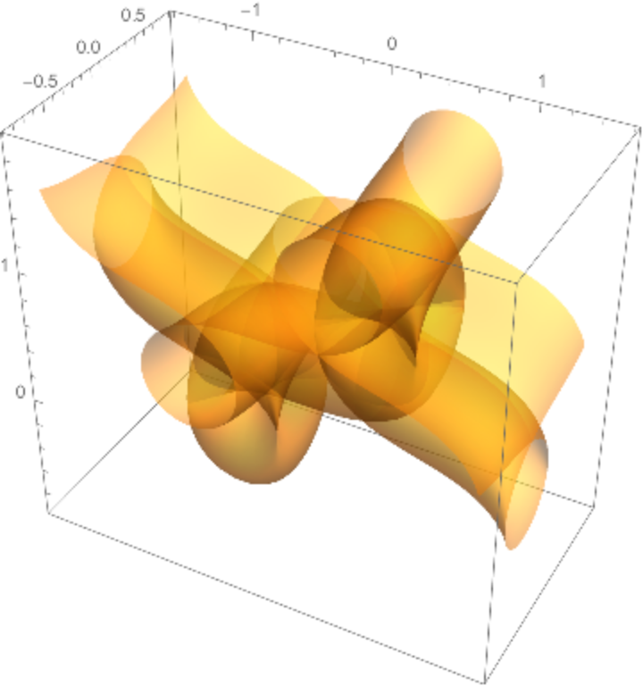
Plot the surface:
| In[20]:= |
![ParametricPlot3D[
Evaluate@
ResourceFunction["TranslationSurface"][Insert[f[t], 0, 2], Insert[g[t], 0, 1], {t, u, v}], {u, -4., 4.}, {v, -2., 2.}, Mesh -> False, PlotPoints -> 80, MaxRecursion -> 5, PlotStyle -> Opacity[.5]]](https://www.wolframcloud.com/obj/resourcesystem/images/15c/15c94274-7ca5-403d-a837-136094161702/0133728ef8dd565e.png)
|
| Out[20]= |
|
This work is licensed under a Creative Commons Attribution 4.0 International License