Wolfram Function Repository
Instant-use add-on functions for the Wolfram Language
Function Repository Resource:
Plot polygons after iteratively applying a translation, scaling and rotation
ResourceFunction["IteratedAffinePlot"][rules, init] plots the polygon described by the points init, and the transformed shape after applying the transformation given by rules. | |
ResourceFunction["IteratedAffinePlot"][rules, init,iter] plots the polygon described by the points init, and the transformed shape after applying the transformation given by rules, for the number of iterations specified by iter. |
| n | all iterations through n |
| {{n}} | plot only the nth iteration |
| {n1,n2} | plots iterations from n1 through n2 |
| {n1,n2,dn} | plots iterations from n1 through n2 in steps of dn |
Show a single iteration of a given set of transformation rules, along with the initial polygon:
| In[1]:= |
| Out[1]= | 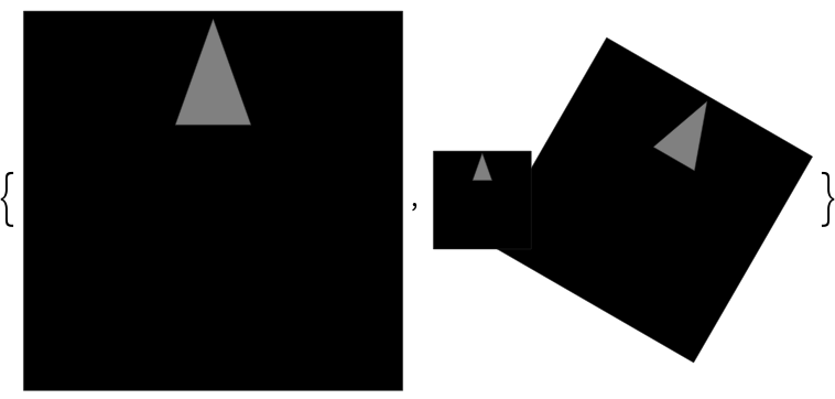 |
Show 5 iterations of a set of transformation rules:
| In[2]:= |
| Out[2]= | 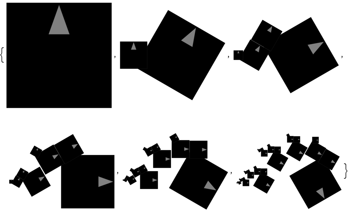 |
Show the fifth through tenth iterations:
| In[3]:= |
| Out[3]= | 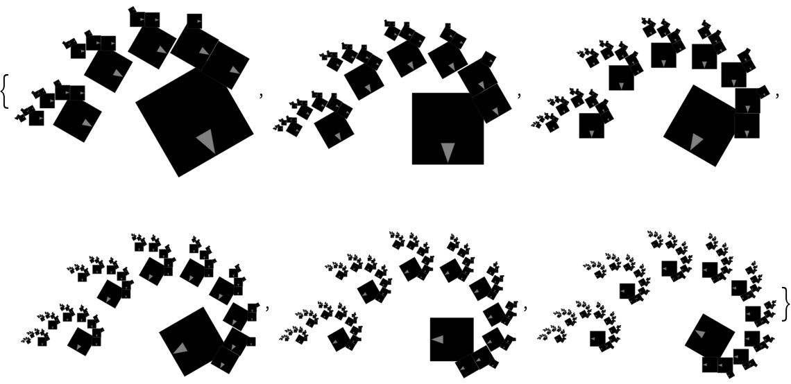 |
Show the fifth, seventh and ninth iterations:
| In[4]:= | ![ResourceFunction[
"IteratedAffinePlot"][{{{1/2, 1/2}, 0.85, 30 \[Degree]}, {{-.1, .5}, .35, 0}}, {{0, 0}, {1, 0}, {1, 1}, {0, 1}}, {5, 10, 2}]](https://www.wolframcloud.com/obj/resourcesystem/images/159/1591d581-bafd-4791-8c33-07a785ce9faf/261b0f2b31746c15.png) |
| Out[4]= | 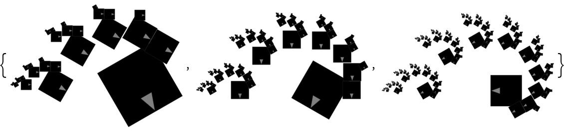 |
Show only the fifth iteration:
| In[5]:= |
| Out[5]= | 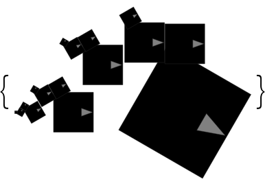 |
Use Graphics options:
| In[6]:= | ![ResourceFunction[
"IteratedAffinePlot"][{{{1/2, 1/2}, 0.85, \[Pi]/6}, {{-.1, .5}, .35, 0}}, {{0, 0}, {1, 0}, {1, 1}, {0, 1}}, {{5}}, Background -> LightBlue, Frame -> True]](https://www.wolframcloud.com/obj/resourcesystem/images/159/1591d581-bafd-4791-8c33-07a785ce9faf/770a60a1cfc267b6.png) |
| Out[6]= | 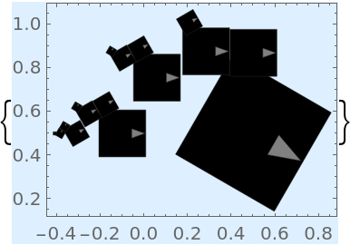 |
The Sierpinski triangle:
| In[8]:= | ![ResourceFunction[
"IteratedAffinePlot"][{{{1/4, 1/(4 Sqrt[3])}, 0.5, 0}, {{1/2, 1/Sqrt[3]}, 0.5, 0}, {{3/4, 1/(4 Sqrt[3])}, 0.5, 0}}, {{0, 0}, {1, 0}, {1/2, Sqrt[3]/2}}, {{4}}, "ShowMarker" -> False] // First](https://www.wolframcloud.com/obj/resourcesystem/images/159/1591d581-bafd-4791-8c33-07a785ce9faf/303d3ffc496a7496.png) |
| Out[8]= | 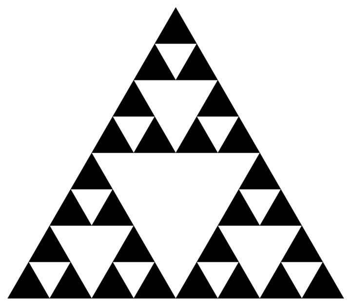 |
Compare with the result of SierpinskiMesh:
| In[9]:= |
| Out[9]= | 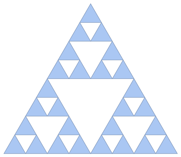 |
The Sierpinski carpet:
| In[10]:= | ![ResourceFunction[
"IteratedAffinePlot"][{{{1/6, 5/6}, 1/3, 0}, {{1/2, 5/6}, 1/3, 0}, {{5/6, 5/6}, 1/3, 0}, {{1/6, 1/2}, 1/3, 0}, {{5/6, 1/2}, 1/3, 0}, {{1/6, 1/6}, 1/3, 0}, {{1/2, 1/6}, 1/3, 0}, {{5/6, 1/6}, 1/3, 0}}, {{0, 0}, {1, 0}, {1, 1}, {0, 1}}, {{4}}, "ShowMarker" -> False] // First](https://www.wolframcloud.com/obj/resourcesystem/images/159/1591d581-bafd-4791-8c33-07a785ce9faf/06091de134ed306a.png) |
| Out[10]= | 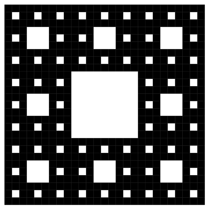 |
Compare with the result of MengerMesh:
| In[11]:= |
| Out[11]= | 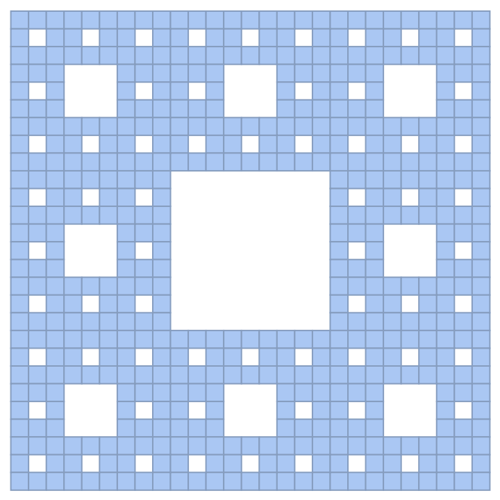 |
This work is licensed under a Creative Commons Attribution 4.0 International License
![ResourceFunction[
"IteratedAffinePlot"][{{{1/2, 1/2}, 0.85, 30 \[Degree]}, {{-.1, .5}, .35, 0}}, {{0, 0}, {1, 0}, {1, 1}, {0, 1}}, {5, 10, 2}, "ShowMarker" -> False]](https://www.wolframcloud.com/obj/resourcesystem/images/159/1591d581-bafd-4791-8c33-07a785ce9faf/3c3543b64c892705.png)
