Wolfram Function Repository
Instant-use add-on functions for the Wolfram Language
Function Repository Resource:
Fit an ellipse to a list of 2D points
ResourceFunction["EllipseFit"][{{x1,y1},{x2,y2},…,{xn,yn}},{x,y}] returns an equation in x and y of an ellipse that fits the given 2D data. |
| TimeConstraint | 1 | the maximum time spent computing exact Eigenvectors before switching to precision specified by the WorkingPrecision option |
| WorkingPrecision | MachinePrecision | the precision used within Eigenvectors after surpassing the TimeConstraint |
Make some 2D data approximating an ellipse:
| In[1]:= | ![data = {{0.92, -0.1}, {1.44, -0.08}, {2.04, 0.4}, {1.2, 0.76}, {1.08, -0.1}, {1.88, 0.7}, {0.48, 0.18}, {0.56, 0.06}, {0.72, 0.5}, {0.9, -0.1}, {0.48, 0.18}, {1.86, 0.72}, {1.18, 0.76}, {0.54, 0.16}, {1.34, 0.74}, {1.76, 0.1}, {2.02, 0.64}, {1.94, 0.16}, {0.54, 0.02}, {1.04, -0.14}, {0.52, 0.12}, {1.72, 0.06}, {1.12, -0.1}, {1.38, -0.08}, {1.32, -0.1}, {1.0, -0.1}, {1.98, 0.28}, {0.54, 0.3}, {0.98, 0.66}, {1.64, 0.76}, {1.78, 0.76}, {1.64, 0.0}, {0.54`, 0.38`}, {1.2, 0.76}, {1.4, 0.74}, {1.1, -0.14}, {0.64, 0.46}, {1.32, -0.08}, {0.54, 0.4}};
ListPlot[data, AspectRatio -> Automatic, Frame -> True, Axes -> False]](https://www.wolframcloud.com/obj/resourcesystem/images/14d/14d377bc-7c9f-42c7-b9b2-caa98965c565/234930ce80164217.png) |
| Out[2]= | 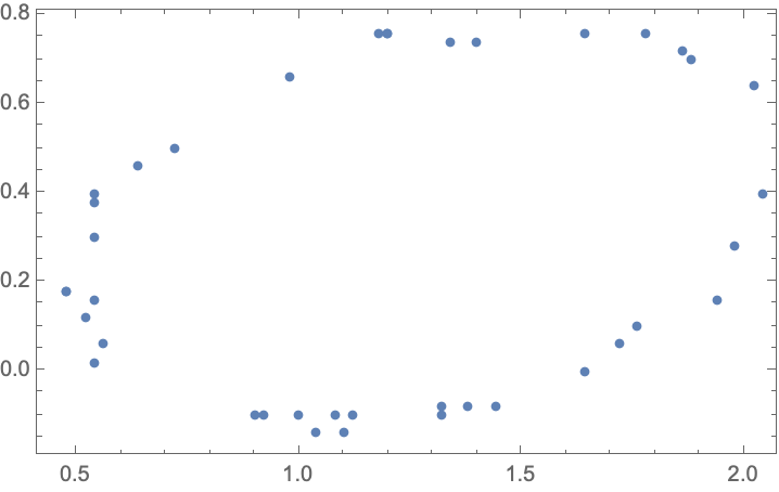 |
EllipseFit returns the equation of the ellipse that best approximates the data:
| In[3]:= |
| Out[4]= |
Plot the ellipse and the data:
| In[5]:= |
| Out[5]= | 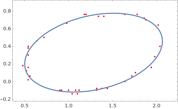 |
EllipseFit works well when the data is over only a part of an ellipse:
| In[6]:= | ![data = {{-0.99, 0.58}, {-1.27, 0.52}, {-1.55, 0.45}, {-1.82, 0.39}, {-2.09, 0.32}, {-2.34, 0.24}, {-2.57, 0.17}, {-2.79, 0.1}, {-3.0, 0.02}, {-3.19, -0.05}, {-3.36, -0.13}, {-3.51, -0.2}, {-3.65, -0.27}, {-3.76, -0.34}, {-3.85`, -0.41}, {-3.92, -0.48}, {-3.97, -0.54}, {-4.0, -0.61}, {-4.0, -0.66}, {-3.98, -0.72}, {-3.9, -0.77}} ;
fit = ResourceFunction[
"EllipseFit", ResourceSystemBase -> "https://www.wolframcloud.com/obj/resourcesystem/api/1.0"][data, {x, y}];
ContourPlot[Evaluate@fit, {x, -4, 2.2}, {y, -1, 1}, AspectRatio -> Automatic, Prolog -> {AbsolutePointSize@5, Red, Point@data}, ImageSize -> {700, 250}]](https://www.wolframcloud.com/obj/resourcesystem/images/14d/14d377bc-7c9f-42c7-b9b2-caa98965c565/66543930ff356dd8.png) |
| Out[9]= | 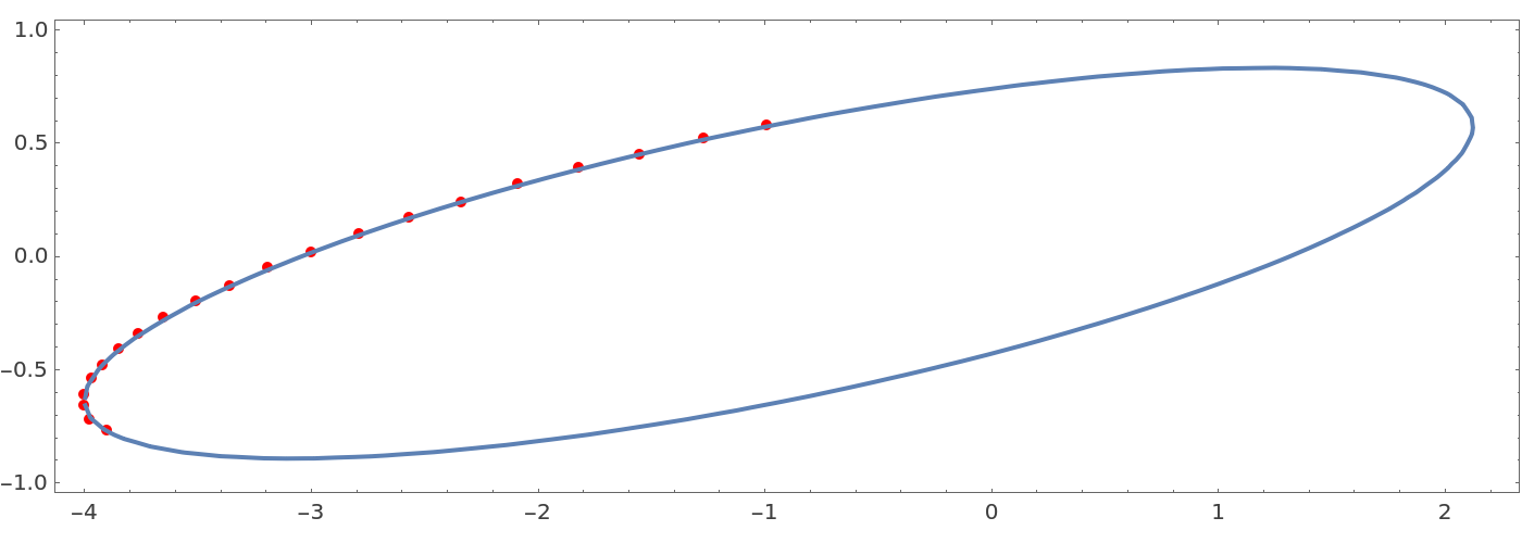 |
This data has 50 digits of precision and EllipseFit finds the equation of an ellipse with all the precision that can be justified:
| In[10]:= |
| Out[11]= |  |
The above curve has 45.2 digits of precision. Almost five digits of precision were lost in finding the equation of this ellipse:
| In[12]:= |
| Out[12]= |
In this case the data is exact and we get the equation of an ellipse with exact coefficients. Whenever all the data is exact and not all the data is exactly on an ellipse EllipseFit returns an equation with exact coefficients:
| In[13]:= | ![Clear[x, y];
data = {{1, 2}, {3, 5}, {5, -6}, {7, 28}, {9, -2}};
ResourceFunction[
"EllipseFit", ResourceSystemBase -> "https://www.wolframcloud.com/obj/resourcesystem/api/1.0"][data, {x, y}]](https://www.wolframcloud.com/obj/resourcesystem/images/14d/14d377bc-7c9f-42c7-b9b2-caa98965c565/5e7081b70496cd88.png) |
| Out[15]= |  |
This data is exact and all the points are exactly on an ellipse:
| In[16]:= |
| Out[16]= |  |
With the default setting TimeConstraint→1, this example resorts to numeric computation:
| In[17]:= |
| Out[18]= |
Plot the ellipse and the data:
| In[19]:= |
| Out[19]= | 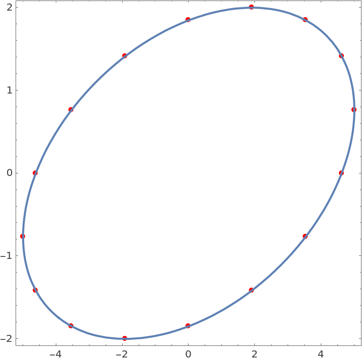 |
With the setting TimeConstraint → ∞, EllipseFit finds an exact solution after several seconds. This would take an extremely long time and require huge amounts of memory if the data had many samples:
| In[20]:= |
| Out[20]= |
This data is exact and all the points are exactly on an ellipse:
| In[21]:= |
| Out[21]= |  |
In this case, EllipseFit switches to arithmetic with 25 digits of precision after exact arithmetic took longer than the TimeConstraint value:
| In[22]:= |
| Out[22]= |
When the data is used for the left side of the equation above we get a value within 10-24 of zero. If the equation had MachinePrecision coefficients, the values below would be within about 10-16 of zero:
| In[23]:= |
| Out[23]= |
With the setting WorkingPrecision→ ∞, EllipseFit finds an exact solution after several seconds. This would take an extremely long time and require huge amounts of memory if the data had many samples:
| In[24]:= |
| Out[24]= |
This data would perfectly fit a hyperbola:
| In[25]:= | ![data = N[{{1/4, 4}, {1/8, 8}, {1/12, 12}, {1/16, 16}, {1/2, 2}, {4, 1/4}, {8, 1/8}, {12, 1/12}, {18, 1/18}, {25, 1/25}}];
ListPlot[data, Frame -> True, Axes -> False, AspectRatio -> Automatic]](https://www.wolframcloud.com/obj/resourcesystem/images/14d/14d377bc-7c9f-42c7-b9b2-caa98965c565/61b6813fcac34197.png) |
| Out[26]= | 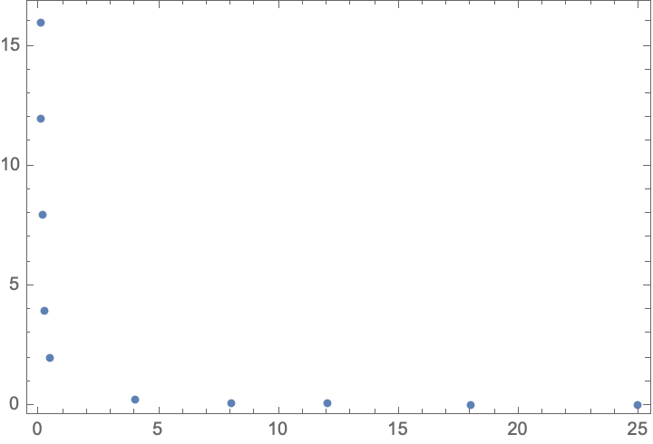 |
EllipseFit finds a curve to fit the data:
| In[27]:= |
| Out[28]= |
Whenever EllipseFit finds a curve to fit the data, the curve is guaranteed to be an ellipse. The plot below shows that the above curve is an ellipse, and it fits the data about as well as an ellipse can fit this data:
| In[29]:= |
| Out[29]= | 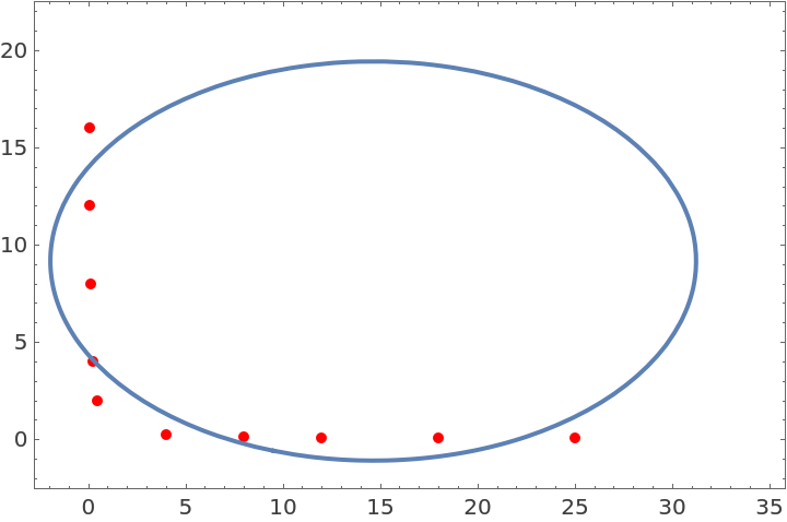 |
EllipseFit fails if the points in the data are nearly along a line or exactly along a line:
| In[30]:= | ![Clear[x, y];
ResourceFunction[
"EllipseFit", ResourceSystemBase -> "https://www.wolframcloud.com/obj/resourcesystem/api/1.0"][{{1.0, 2.0}, {3.0, 4.0001}, {5.0, 6.0003}, {7.0, 7.99998}, {9.0, 9.9996}, {11.0, 12.00002}, {13.0, 14.0006}}, {x, y}]](https://www.wolframcloud.com/obj/resourcesystem/images/14d/14d377bc-7c9f-42c7-b9b2-caa98965c565/0a6dd7a654f47056.png) |
| Out[31]= |
In this case the data has three distinct points, so an infinite collection of ellipses pass perfectly through all the data. When that happens EllipseFit displays a Message and returns unevaluated:
| In[32]:= |
| Out[33]= |
Plot an ellipse:
| In[34]:= |
| Out[34]= | 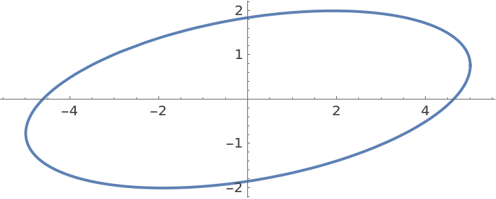 |
Make a list of 200,000 MachinePrecision points near the above ellipse:
| In[35]:= | ![data = Most@
Table[{5 Cos[t], 2 Sin[t + \[Pi]/8]}, {t, 0.0, 2 \[Pi], \[Pi]/100000}] + RandomReal[{-0.2, 0.2}, {200000, 2}];
Dimensions[data]](https://www.wolframcloud.com/obj/resourcesystem/images/14d/14d377bc-7c9f-42c7-b9b2-caa98965c565/77c9dc7af3d91a7d.png) |
| Out[36]= |
EllipseFit finds the ellipse that fits the large list of points in less than 0.1 second:
| In[37]:= |
| Out[38]= |
A plot of the ellipse found looks exactly like the ellipse above:
| In[39]:= |
| Out[39]= | 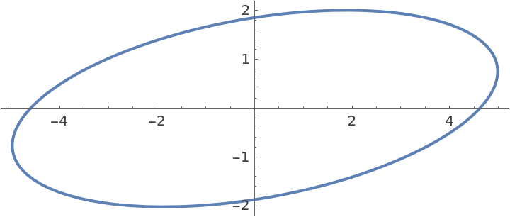 |
Wolfram Language 13.0 (December 2021) or above
This work is licensed under a Creative Commons Attribution 4.0 International License