Wolfram Function Repository
Instant-use add-on functions for the Wolfram Language
Function Repository Resource:
Evaluate the piecewise spherical linear interpolant of given data
ResourceFunction["SphericalLinearInterpolation"][data,t] finds a piecewise spherical linear interpolation of data at the point t. | |
ResourceFunction["SphericalLinearInterpolation"][data] represents an operator form of ResourceFunction["SphericalLinearInterpolation"] that can be applied to an expression. |
Generate some data over a sphere of radius 3:
| In[1]:= |
![vecs = 3 (Normalize /@ RandomVariate[NormalDistribution[], {5, 3}]);
vals = FoldList[Plus, 0, Normalize[VectorAngle @@@ Partition[vecs, 2, 1], Total]];
data = Transpose[{vals, vecs}]](https://www.wolframcloud.com/obj/resourcesystem/images/138/138d6e06-de10-4b4c-8b6f-31c18a72cd06/6e58ffd12ffd1913.png)
|
| Out[1]= |
|
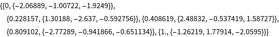
Evaluate the piecewise spherical linear interpolant of the data at a given value:
| In[2]:= |
|
| Out[2]= |
|
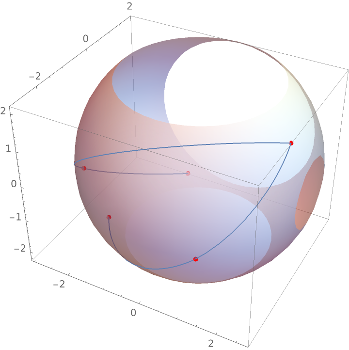
Plot the piecewise spherical linear interpolant along with the original data:
| In[3]:= |
![Show[ParametricPlot3D[
ResourceFunction["SphericalLinearInterpolation"][data, t], {t, 0, 1}], Graphics3D[{{Opacity[0.6], Sphere[{0, 0, 0}, 3]}, {Red, AbsolutePointSize[5], Point[vecs]}}]]](https://www.wolframcloud.com/obj/resourcesystem/images/138/138d6e06-de10-4b4c-8b6f-31c18a72cd06/0e5a86e95a32b3b7.png)
|
| Out[3]= |
|
Evaluate the piecewise spherical linear interpolant for four-dimensional vectors:
| In[4]:= |
|
| Out[4]= |
|
Evaluate the piecewise spherical linear interpolant for high-precision data:
| In[5]:= |
![data = Transpose[{N[Subdivide[4], 20], Normalize /@ RandomVariate[NormalDistribution[], {5, 3}, WorkingPrecision -> 20]}];
ResourceFunction["SphericalLinearInterpolation"][data, 1/2]](https://www.wolframcloud.com/obj/resourcesystem/images/138/138d6e06-de10-4b4c-8b6f-31c18a72cd06/540c8d6e5a82c386.png)
|
| Out[5]= |
|
A function for taking a bounded random step on a sphere:
| In[6]:= |
![boundedRandomStep[v_?VectorQ, \[CurlyPhi]_?NumericQ] := RotationMatrix[{{0, 0, 1}, v}].({0, 0, Cos[\[CurlyPhi]]} + Sin[\[CurlyPhi]] Append[
Normalize[RandomVariate[NormalDistribution[], 2]], 0])](https://www.wolframcloud.com/obj/resourcesystem/images/138/138d6e06-de10-4b4c-8b6f-31c18a72cd06/61626c12ca81af01.png)
|
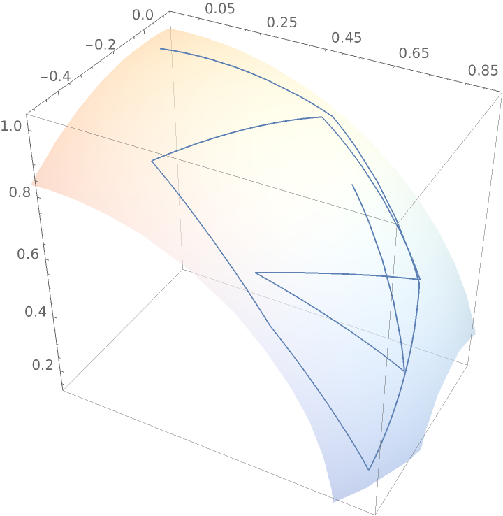
Visualize a random walk with bounded steps on a sphere:
| In[7]:= |
![steps = NestList[boundedRandomStep[#, \[Pi]/6] &, {0, 0, 1}, 10];
vals = FoldList[Plus, 0, Normalize[VectorAngle @@@ Partition[steps, 2, 1], Total]];
data = Transpose[{vals, steps}];
Show[ParametricPlot3D[
ResourceFunction["SphericalLinearInterpolation"][data, t], {t, 0, 1}], Graphics3D[{Opacity[0.6], Sphere[]}]]](https://www.wolframcloud.com/obj/resourcesystem/images/138/138d6e06-de10-4b4c-8b6f-31c18a72cd06/7e2f5bd821d7ee7f.png)
|
| Out[7]= |
|
This work is licensed under a Creative Commons Attribution 4.0 International License