Details and Options
This uses the generalized aggregation model from A New Kind of Science Chapter 7.
Neighborhood configurations are as specified by an outer totalistic cellular automaton rule.
While entering the rule number, one must make sure that "Dimension" is set to 2.
Possible forms for rule are:
| {n,{2,1},{1,1}} | 9-neighbor totalistic rule |
| {n,{2,{{0,1,0},{1,1,1},{0,1,0}}},{1,1}} | 5-neigbbor totalistic rule |
| {n,{2,{{0,2,0},{2,1,2},{0,2,0}}},{1,1}} | 5-neighbor outer totalistic rule |
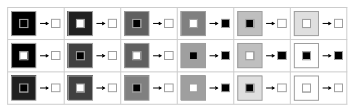
The following keys can be used to specify a rule given as an association:
| "TotalisticCode" | n | totalistic code |
| "OuterTotalisticCode" | n | outer totalistic code |
| "Dimension" | d | overall dimension (always 2) |
| "Neighborhood" | type | neigborhood |
| "Range" | r | range of rule |
| "Colors" | k | number of colors |
| "GrowthCases" | {g1,g2,…} | make a cell 1 when gi of its neighbors are 1 |
| "GrowthSurvivalCases" | {{g1,…},{s1,…}} | 1 for gi neighbors; unchanged for si |
| "GrowthDecayCases" | {{g1,…},{d1,…}} | 1 for gi neighbors; 0 for di |
Possible settings for "Neighborhood" include:
5 or "VonNeumann"
9 or "Moore"
The number of possible aggregation system rules is as follows:
| 2D general rules | 2512 |
| 2D 9-neighbor totalistic rules | 210 |
| 2D 5-neighbor totalistic rules | 26 |
| 2D 5-neighbor outer totalistic rules | 210 |
| 2D outer totalistic rules | 217+1 |
The initial condition specification should be of the form aspec, {aspec,bspec} or {{{aspec1,off1},{aspec2,off2},…,{aspecn,offn}},bspec} (for n>0). Each aspec must be a non-empty array of rank 2 whose elements at level 2 are integers i in the range 0≤i≤"Colors"-1 ("Colors"=2 by default).
t should be a natural number. If t is specified as a list of a certain depth, then the first element of the flattened list will be taken as the input.
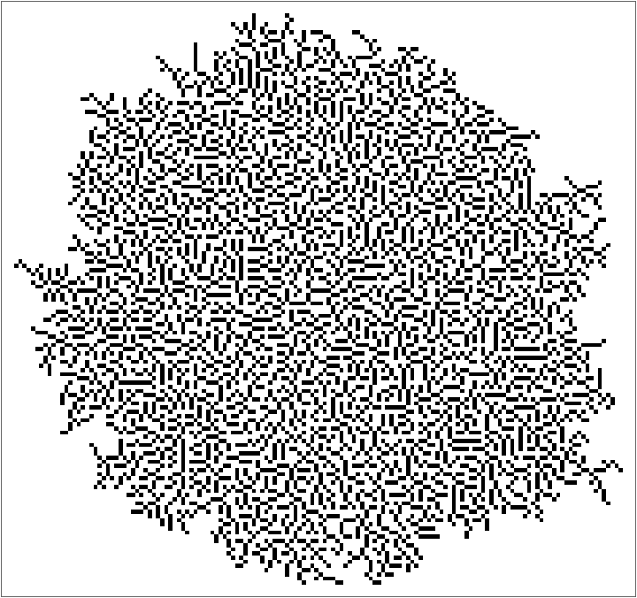
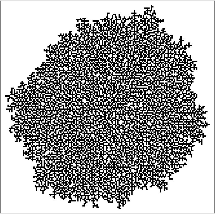
![ArrayPlot@
ResourceFunction[
"AggregationSystem"][<|"OuterTotalisticCode" -> 4, "Dimension" -> 2, "Neighborhood" -> 5|> , CenterArray[1, {1, 1}], 10000]](https://www.wolframcloud.com/obj/resourcesystem/images/065/065444d6-7339-44a4-8688-beddebf133e7/472151b2b665db46.png)
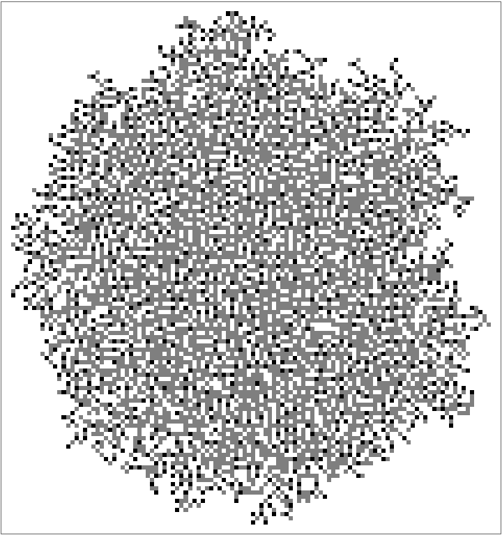
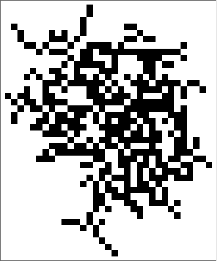
![ArrayPlot[
ResourceFunction[
"AggregationSystem"][<|"Dimension" -> 2, "GrowthCases" -> {3, 6, 2}|>, {{1, 1, 1, 1, 1} {1, 0, 1, 1, 1}, {1,
0, 0, 1, 1}}, 20000]]](https://www.wolframcloud.com/obj/resourcesystem/images/065/065444d6-7339-44a4-8688-beddebf133e7/1fa6ffabae918282.png)
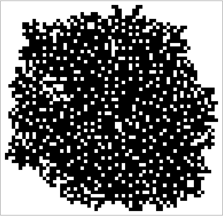
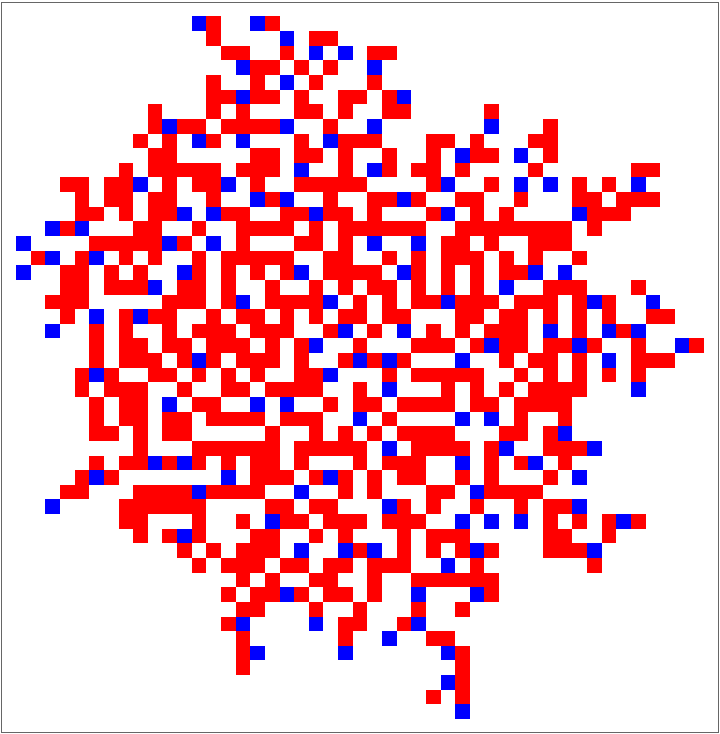
![ArrayPlot[
ResourceFunction[
"AggregationSystem"][<|"TotalisticCode" -> 344, "Dimension" -> 2, "Colors" -> 4|> , CenterArray[1, {1, 1}], 1000], ColorRules -> {1 -> Red, 2 -> Blue}]](https://www.wolframcloud.com/obj/resourcesystem/images/065/065444d6-7339-44a4-8688-beddebf133e7/3b1d7dafd6256151.png)