Wolfram Function Repository
Instant-use add-on functions for the Wolfram Language
Function Repository Resource:
Evaluate an infinite sum using the Levin transformation
ResourceFunction["LevinSum"][f,{i,imin,∞}] numerically evaluates the sum |
| "ExtraTerms" | 15 | number of terms to use in the Levin transform |
| "Terms" | 15 | number of terms to sum directly |
| "Type" | Automatic | the type of Levin transformation to use |
| WorkingPrecision | MachinePrecision | the precision used in internal computations |
| "T" | t-transformation, gn=Sn-Sn-1 |
| "U" | u-transformation, gn=(n+1)(Sn-Sn-1) |
| "V" | v-transformation, gn=-(Sn+1-Sn)(Sn-Sn-1)/(Sn+1-2Sn+Sn-1) |
| "D" | d-transformation, gn=Sn+1-Sn |
Evaluate the alternating harmonic series:
| In[1]:= |
| Out[1]= |
Compare with the closed form:
| In[2]:= |
| Out[2]= |
Use 25 terms for the Levin transformation:
| In[3]:= |
| Out[3]= |
Compare with the exact result:
| In[4]:= |
| Out[4]= |
Set "Terms" to 0 so that all terms are used in extrapolation:
| In[5]:= |
| Out[5]= |
Compare with the exact result:
| In[6]:= |
| Out[6]= |
Directly sum the first 25 terms before applying the Levin transformation:
| In[7]:= |
| Out[7]= |
Compare with the exact result:
| In[8]:= |
| Out[8]= |
Show the results of the different Levin transformations on an alternating series:
| In[9]:= | ![TableForm[
Table[With[{r = ResourceFunction["LevinSum"][(-1)^k/(
2 k + 1), {k, 0, \[Infinity]}, "Type" -> t, WorkingPrecision -> 25]}, {t, r, r - \[Pi]/4}], {t, {"T", "U", "V", "D"}}], TableHeadings -> {None, {"Type", "Result", "Error"}}]](https://www.wolframcloud.com/obj/resourcesystem/images/03f/03f0f6e9-dca6-4105-8bf4-a46ea3dfd8f7/6f60c987497a2bb0.png) |
| Out[9]= |  |
Show the results of the different Levin transformations on a non-alternating series:
| In[10]:= | ![TableForm[
Table[With[{r = ResourceFunction["LevinSum"][1/k^2, {k, 1, \[Infinity]}, "Type" -> t, WorkingPrecision -> 25]}, {t, r, r - \[Pi]^2/6}], {t, {"T", "U", "V", "D"}}], TableHeadings -> {None, {"Type", "Result", "Error"}}]](https://www.wolframcloud.com/obj/resourcesystem/images/03f/03f0f6e9-dca6-4105-8bf4-a46ea3dfd8f7/439b740bc0cf2dfd.png) |
| Out[10]= |  |
Use a higher setting of WorkingPrecision:
| In[11]:= |
| Out[11]= |
Compare with the exact result:
| In[12]:= |
| Out[12]= |
Use the Levin d-transform to evaluate the Dirichlet eta function:
| In[13]:= |
Compare with the built-in DirichletEta:
| In[14]:= |
| Out[14]= | 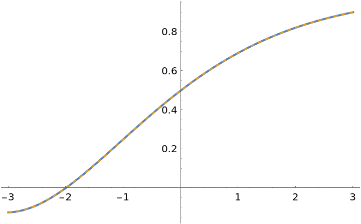 |
Plot the relative error:
| In[15]:= |
| Out[15]= | 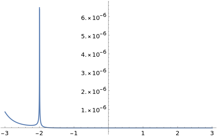 |
Use the Levin v-transform with NIntegrate to numerically evaluate an oscillatory integral:
| In[16]:= | ![term[j_Integer] := NIntegrate[
BesselJ[0, x], {x, BesselJZero[0, j], BesselJZero[0, j + 1]}, WorkingPrecision -> 25]
NIntegrate[BesselJ[0, x], {x, 0, BesselJZero[0, 1]}, WorkingPrecision -> 25] + ResourceFunction["LevinSum"][term[j], {j, 1, \[Infinity]}, "Type" -> "V", WorkingPrecision -> 25]](https://www.wolframcloud.com/obj/resourcesystem/images/03f/03f0f6e9-dca6-4105-8bf4-a46ea3dfd8f7/5669c80cb03e98b5.png) |
| Out[16]= |
Compare with the exact result:
| In[17]:= |
| Out[17]= |
Directly summing the first few terms of a series usually does not give sufficient accuracy:
| In[18]:= |
| Out[18]= |
| In[19]:= |
| Out[19]= |
Using the Levin transform on a series often gives better results:
| In[20]:= |
| Out[20]= |
| In[21]:= |
| Out[21]= |
LevinSum may give finite results for formally divergent series:
| In[22]:= |
| Out[22]= |
Compare with the exact result:
| In[23]:= |
| Out[23]= |
Numerically evaluate a formally divergent oscillatory integral:
| In[24]:= |
| Out[24]= |
Compare with the exact answer:
| In[25]:= |
| Out[25]= |
| In[26]:= |
| Out[26]= |
This work is licensed under a Creative Commons Attribution 4.0 International License