Wolfram Language Paclet Repository

Community-contributed installable additions to the Wolfram Language

Primary Navigation

    • Cloud & Deployment
    • Core Language & Structure
    • Data Manipulation & Analysis
    • Engineering Data & Computation
    • External Interfaces & Connections
    • Financial Data & Computation
    • Geographic Data & Computation
    • Geometry
    • Graphs & Networks
    • Higher Mathematical Computation
    • Images
    • Knowledge Representation & Natural Language
    • Machine Learning
    • Notebook Documents & Presentation
    • Scientific and Medical Data & Computation
    • Social, Cultural & Linguistic Data
    • Strings & Text
    • Symbolic & Numeric Computation
    • System Operation & Setup
    • Time-Related Computation
    • User Interface Construction
    • Visualization & Graphics
    • Random Paclet
    • Alphabetical List
  • Using Paclets
    • Get Started
    • Download Definition Notebook
  • Learn More about Wolfram Language

QuantumFramework

Tutorials

  • Getting Started

Guides

  • Wolfram Quantum Computation Framework

Tech Notes

  • Bell's Theorem
  • Circuit Diagram
  • Exploring Fundamentals of Quantum Theory
  • Quantum object abstraction
  • Quantum Optimization
  • Second Quantization Functions
  • Tensor Network
  • Quantum Computation

Symbols

  • QuantumBasis
  • QuantumChannel
  • QuantumCircuitMultiwayGraph [EXPERIMENTAL]
  • QuantumCircuitOperator
  • QuantumDistance
  • QuantumEntangledQ
  • QuantumEntanglementMonotone
  • QuantumEvolve
  • QuantumMeasurement
  • QuantumMeasurementOperator
  • QuantumMeasurementSimulation
  • QuantumMPS [EXPERIMENTAL]
  • QuantumOperator
  • QuantumPartialTrace
  • QuantumPhaseSpaceTransform
  • QuantumShortcut [EXPERIMENTAL]
  • QuantumStateEstimate [EXPERIMENTAL]
  • QuantumState
  • QuantumTensorProduct
  • QuantumWignerMICTransform [EXPERIMENTAL]
  • QuantumWignerTransform [EXPERIMENTAL]
  • QuditBasis
  • QuditName
Quantum Optimization
Quantum Natural Gradient Descent
Examples Custom Functions
Quantum Linear Solver
​
In this Tech Note, we document the implementation and utilization of essential functions used in the
Wolfram Language Example Repository
for Quantum Optimization algorithms.
By providing a comprehensive overview and usage guidelines for these functions, we aim to introduce new and experienced users into quantum optimization techniques and quantum computing research.
In[92]:=
<<Wolfram`QuantumFramework`QuantumOptimization`
Quantum Natural Gradient Descent
Gradient-based optimization methods represent a cornerstone in the field of numerical optimization, offering powerful techniques to minimize or maximize objective functions in various domains, ranging from machine learning and deep learning to physics and engineering. These methods utilize the gradient, or derivative, of the objective function with respect to its parameters to iteratively update them in a direction that reduces the function's value.
This Tech Note will include a brief introduction to the Fubini-Study metric tensor and Quantum Natural Gradient Descent. We will provide illustrative examples and compare these methods to regular gradient descent algorithms.

FubinyStudyMetricTensor

FubiniStudyMetricTensor[QuantumState[...] ,opts]
calculates the Fubini–Study metric tensor as defined by the VQE approach from a QuantumState with defined parameters
The Fubini-Study metric tensor plays a crucial role in Quantum Natural Gradient Descent. Originating from the field of differential geometry, the Fubini-Study metric tensor enables the quantification of distances between quantum states on the complex projective Hilbert space.
In the context of Quantum Natural Gradient Descent, this metric tensor serves as a fundamental tool for characterizing the geometry of the parameter space associated with parameterized quantum circuits. By incorporating the Fubini-Study metric tensor into the optimization process, this algorithm effectively accounts for the curvature of the quantum state manifold, enabling more precise and efficient updates of circuit parameters.
Considering a variational state ϕ(θ), their correspondant Fubiny-Study metric follows:
g
ij
=Re
∂
i
ϕ

∂
j
ϕ
-
∂
i
ϕ

ϕ

ϕ

∂
j
ϕ
​​
where
|
∂
i
ϕ(θ)〉=
∂
i
|ϕ(θ)〉/∂
θ
i
.

Example

Implement a simple single qubit state:
In[3]:=
state=
QuantumState
[{Cos[θ1],Exp[2*I*θ2]*Sin[θ1]},"Parameters"{θ1,θ2}]
Out[3]=
QuantumState
Pure state
Qudits: 1
Type: Vector
Dimension: 2

In[4]:=
state["Formula"]
Out[4]=
Cos[θ1]|0〉+
2θ2

Sin[θ1]|1〉
Apply the FubiniStudyMetricTensor function to obtain the calculated QuantumOperator:
In[5]:=
FubiniStudyMetricTensor[state]
Out[5]=
QuantumOperator
Pure map
​
Dimension: 2→2
Order: {1}→{1}

In[6]:=
FubiniStudyMetricTensor[state,"MatrixForm"]
Out[6]//MatrixForm=
1
0
0
2
Sin[2θ1]

Properties

QuantumNaturalGradientDescent

Quantum Natural Gradient-Based Optimization Methods represent a cutting-edge approach to optimizing parameterized quantum circuits in the field of quantum computing. Unlike classical gradient-based methods, Quantum Natural Gradient techniques account for the unique geometry of the quantum state manifold, mitigating issues such as barren plateaus and enabling faster convergence rates.
An optimization step in a gradient descent is given by:
θ
t+1
=
θ
t
-η∇ℒ(θ)
where ℒ(θ) is the cost function with parameters θ, and η is the step rate. Each step in this approach assumes a flat Euclidean space, which would lead us to not–unique parametrizations that can disrupt our optimization, specially in singular points. In order to avoid this problem we must use non-Euclidean parameter spaces, performing what is called a natural gradient descent.
The quantum state space features an invariant metric tensor referred to as the Fubini–Study metric tensor
g
ij
, which can be used to develop a quantum version of a natural gradient descent. Then each optimization step is given by:
θ
t+1
=
θ
t
-η
+
g
(θ)∇ℒ(θ)
where
+
g
the Fubini-Study metric tensor pseudo-inverse.
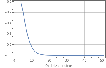
QuantumNaturalGradientDescent[f,metric ,opts]
calculates the gradient descent of f using the defined metric tensor for the parameters space.
We will briefly demonstrate how to apply all these functions in Wolfram quantum framework.
QuantumNaturalGradientDescent function follows the fundamental process of the Variational Quantum Eigensolver (VQE) which involves using a brief quantum circuit U(θ), characterized by parameters
θ={
θ
1
,…
θ
m
}
to iteratively adjust θ to minimize the average energy or cost function:
f(θ)=〈ϕ(θ)|H|ϕ(θ)〉
for the ansatz
|ϕ(θ)〉=U(θ)|0〉
.

Example

Implement a simple single qubit state:
In[3]:=
state=
QuantumState
[{Cos[θ1],Exp[2*I*θ2]*Sin[θ1]},"Parameters"{θ1,θ2}];
In[4]:=
state["Formula"]
Out[4]=
Cos[θ1]|0〉+
2θ2

Sin[θ1]|1〉
Calculate the Fubiny-Study metric tensor:
In[4]:=
metric=FubiniStudyMetricTensor[state]
Out[4]=
QuantumOperator
Pure map
​
Dimension: 2→2
Order: {1}→{1}

In[6]:=
FubiniStudyMetricTensor[state,"Matrix"]
Out[6]=
{{1,0},{0,
2
Sin[2θ1]
}}
Calculate a
|ϕ(θ)〉
state vector:
In[5]:=
|
ϕ
〉
=state["StateVector"];
〈
ϕ
|
=
†
state
["StateVector"];
Implement a cost function 〈ϕ(θ)|H |ϕ(θ)〉 :
In[6]:=
cost[θ1_,θ2_]=
〈
ϕ
|
.PauliMatrix[1].
|
ϕ
〉
;
In[7]:=
FullSimplify[cost[θ1,θ2],{θ1,θ2}∈Reals]
Out[7]=
Cos[2θ2]Sin[2θ1]
Use QuantumNaturalGradientDescent to minimize the function:
In[12]:=
qp=
QuantumNaturalGradientDescent
[cost,metric,"InitialPoint"{π/12,π/12},"LearningRate"0.05];
QuantumNaturalGradientDescent returns all the parameters obtained until convergence. We can check how the minimization evolved:
In[13]:=
ListLinePlot[cost@@@qp,FrameLabel{"Optimization steps","f"},​​FrameTrue,GridLinesAutomatic]
Out[13]=
Check optimization results:
In[14]:=
Chop[{#,cost@@#}]&@Last[qp]
Out[14]=
{{0.785368,1.5708},-1.}

Options

"Gradient"
None
indicate correspondant gradient function
∇f
to be used
"InitialPoint"
Automatic
initial starting point for the optimization process
"LearningRate"
0.8
step size taken during each iteration
"MaxIterations"
50
maximum number of iterations to use
Gradient
You can specify the correspondant gradient function
∇f
:
In[15]:=
costgrad[θ1_,θ2_]=Grad[FullSimplify[cost[θ1,θ2],{θ1,θ2}∈Reals],{θ1,θ2}]
Out[15]=
{2Cos[2θ1]Cos[2θ2],-2Sin[2θ1]Sin[2θ2]}
In[16]:=
parameters=
QuantumNaturalGradientDescent
[​​cost,metric,​​"InitialPoint"{π/12,π/12},​​"LearningRate"0.05,​​"Gradient"costgrad];
In[17]:=
Chop[{#,cost@@#}]&@Last[parameters]
Out[17]=
{{0.785368,1.5708},-1.}
If the gradient is not specified, it is calculated numerically using a center finite differnece algorithm.
InitialPoint
Specify the initial point to start the iteration, compare the following gradient descent setups:
Analyze the parameters evolution with different starting point:
LearningRate
Specify step size (η) taken during each iteration, compare the following gradient descent setups:
In this case, the optimization is done almost instantly by "LearningRate"  0.1:
Verify the trajectory generated by "LearningRate"  0.5 and "LearningRate"  0.1:
MaxIterations

Results Overview

Verify the evolution of the paremeters for each case:

GradientDescent

Quantum Linear Solver
We will briefly demonstrate how to apply all these functions in Wolfram quantum framework.

Details and Options

QuantumLinearSolve utilizes a multiplexer-based variational quantum linear solver algorithm. The primary distinctions from a conventional variational quantum linear solver algorithm are as follows:
◼
  • The solution to the linear system is encoded directly in the amplitudes of the resultant quantum state.
  • This approach simplifies the standard variational quantum linear solver by reducing the need for multiple circuits used in the real-imaginary decomposition of the solution and the term-by-term computation within quantum circuits. A detailed step-by-step implementation is outlined in this documentation.
    The basic steps to implement the algorithm are the following:

    Algorithm Implementation

    Ansatz
    Multiplexer
    Cost Function

    Options

    Ansatz
    GlobalPhaseAccuracy
    AccuracyGoal & PrecisionGoal
    Method
    Heuristic methods include:
    Some methods may give suboptimal results for certain problems:
    WorkingPrecision

    Example

    Simple example
    Generate a random 4×4 real matrix:
    Generate a random complex vector of the length 4:
    When running above code, you may see a progress box describing steps and estimated time.
    Compare the results:
    Properties
    You can request the components used during the calculation using a third property argument:
    Show the ansatz quantum state used for parameter optimization"
    Show the quantum circuit used for parameter optimization:
    Request more than one property:
    Examples Custom Functions

    Fubini-Study Metric Tensor (Alternative Methods)

    The Fubini-Study metric tensor plays a crucial role in Quantum Natural Gradient Descent. Originating from the field of differential geometry, the Fubini-Study metric tensor enables the quantification of distances between quantum states on the complex projective Hilbert space. In the context of Quantum Natural Gradient Descent, this metric tensor serves as a fundamental tool for characterizing the geometry of the parameter space associated with parameterized quantum circuits. By incorporating the Fubini-Study metric tensor into the optimization process, this algorithm effectively accounts for the curvature of the quantum state manifold, enabling more precise and efficient updates of circuit parameters.

    Example

    Stochastic Parameter Shift–Rule

    © 2025 Wolfram. All rights reserved.

    • Legal & Privacy Policy
    • Contact Us
    • WolframAlpha.com
    • WolframCloud.com