Wolfram Language Paclet Repository

Community-contributed installable additions to the Wolfram Language
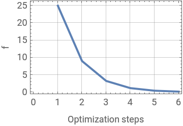
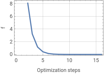
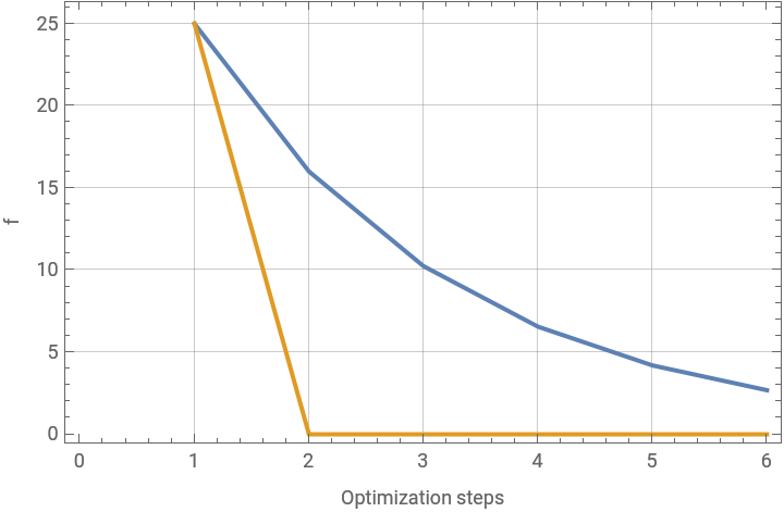
Primary Navigation

    • Cloud & Deployment
    • Core Language & Structure
    • Data Manipulation & Analysis
    • Engineering Data & Computation
    • External Interfaces & Connections
    • Financial Data & Computation
    • Geographic Data & Computation
    • Geometry
    • Graphs & Networks
    • Higher Mathematical Computation
    • Images
    • Knowledge Representation & Natural Language
    • Machine Learning
    • Notebook Documents & Presentation
    • Scientific and Medical Data & Computation
    • Social, Cultural & Linguistic Data
    • Strings & Text
    • Symbolic & Numeric Computation
    • System Operation & Setup
    • Time-Related Computation
    • User Interface Construction
    • Visualization & Graphics
    • Random Paclet
    • Alphabetical List
  • Using Paclets
    • Get Started
    • Download Definition Notebook
  • Learn More about Wolfram Language

QuantumFramework

Tutorials

  • Getting Started

Guides

  • QuantumPhaseSpaceTranform
  • Wolfram Quantum Computation Framework

Tech Notes

  • Bell's Theorem
  • Circuit Diagram
  • Example Repository Functions
  • Exploring Fundamentals of Quantum Theory
  • Quantum object abstraction
  • Tensor Network
  • Quantum Computation

Symbols

  • QuantumBasis
  • QuantumChannel
  • QuantumCircuitMultiwayGraph [EXPERIMENTAL]
  • QuantumCircuitOperator
  • QuantumDistance
  • QuantumEntangledQ
  • QuantumEntanglementMonotone
  • QuantumEvolve
  • QuantumMeasurement
  • QuantumMeasurementOperator
  • QuantumMeasurementSimulation
  • QuantumMPS [EXPERIMENTAL]
  • QuantumOperator
  • QuantumPartialTrace
  • QuantumPhaseSpaceTransform
  • QuantumShortcut [EXPERIMENTAL]
  • QuantumStateEstimate [EXPERIMENTAL]
  • QuantumState
  • QuantumTensorProduct
  • QuantumWignerMICTransform [EXPERIMENTAL]
  • QuantumWignerTransform [EXPERIMENTAL]
  • QuditBasis
  • QuditName
Example Repository Functions
Gradient-Based Optimization Methods
Examples Custom Functions
In this Tech Note, we document the implementation and utilization of essential functions used in the
Wolfram Language Example Repository
for Quantum Computing algorithms. The examples include the Quantum Natural Gradient Descent, Stochastic Parameter Shift Rule and more.
By providing a comprehensive overview and usage guidelines for these functions, we aim to introduce new and experienced users into quantum optimization techniques, quantum machine learning and quantum computing research.
Gradient-Based Optimization Methods
Gradient-based optimization methods represent a cornerstone in the field of numerical optimization, offering powerful techniques to minimize or maximize objective functions in various domains, ranging from machine learning and deep learning to physics and engineering. These methods leverage the gradient, or derivative, of the objective function with respect to its parameters to iteratively update them in a direction that reduces the function's value.
In this Tech Note, we'll provide illustrative examples for both conventional gradient descent and quantum natural gradient descent methods.
GradientDescent[f,{
value
1
,
value
2
,… }, opts]
calculates the gradient descent of f using
value
i
as initial parameters.
QuantumNaturalGradientDescent[f,{
value
1
,
value
2
,… },metric ,opts]
calculates the gradient descent of f using
value
i
as initial parameters and metric as
metric
tensor to define the parameters space.
We will briefly demonstrate how to apply all these functions in Wolfram quantum framework.

GradientDescent

Gradient Descent aims to minimize a given objective function by iteratively updating the parameters in the direction of the steepest descent of the function. This simplicity and effectiveness render Gradient Descent indispensable in the realm of optimization, serving as the basis for numerous advanced optimization algorithms.

Example

Implement a simple function
f[x_,y_]:=
2
x
+
2
y
Set initial parameters and use GradientDescent to minimize the function:
initial={3,4};
parameters=GradientDescent[f,initial];
GradientDescent returns all the parameters obtained until convergence. We can check how the minimization evolved:
ListLinePlot[f@@@parameters,FrameLabel{"Optimization steps","f"},​​FrameTrue,GridLinesAutomatic]
The last parameters obtained correspond to the minimized function:
{f@@#,x#〚1〛,y#〚2〛}&@Last[parameters]
{1.6333×
-21
10
,x2.42484×
-11
10
,y3.23313×
-11
10
}
We can contrast the result using NMinimize:
NMinimize[f[x,y],{x,y}]
{0.,{x0.,y0.}}

Options

"Jacobian"
None
indicate correspondant gradient function
∇f
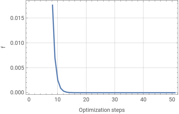
to be used
"MaxIterations"
50
maximum number of iterations to use
"LearningRate"
0.8
step size taken during each iteration
Jacobian
You can specify the correspondant gradient function
∇f
:
df[x_,y_]=
∇
{x,y}
f[x,y]
{2x,2y}
parameters=GradientDescent[f,initial,"Jacobian"df];
{f@@#,x#〚1〛,y#〚2〛}&@Last[parameters]
{1.6333×
-21
10
,x2.42484×
-11
10
,y3.23313×
-11
10
}
If the gradient is not specified, it is calculated numerically using a center finite differnece algorithm.
MaxIterations
Specify the maximum number of iterations to use:
parameters1=GradientDescent[f,initial,"MaxIterations"5];​​parameters2=GradientDescent[f,initial,"MaxIterations"15];
Grid[{​​ListLinePlot[{f@@@#},​​FrameLabel{"Optimization steps","f"},​​FrameTrue,GridLinesAutomatic,ImageSizeSmall]&/@{parameters1,parameters2}}​​]
LearningRate
Specify step size (η) taken during each iteration, compare the following gradient descent setups:
parameters1=GradientDescent[f,initial,"LearningRate"0.9,"MaxIterations"5];​​parameters2=GradientDescent[f,initial,"LearningRate"0.5,"MaxIterations"5];
In this case, the optimization is done almost instantly by "LearningRate"  0.5:
ListLinePlot[{f@@@parameters1,f@@@parameters2},FrameLabel{"Optimization steps","f"},​​PlotLegends{"η = 0.9","η = 0.5"},​​FrameTrue,GridLinesAutomatic]
η = 0.9
η = 0.5
We can visually verify that η = 0.9 was not efficent to find the solution:
ListPlot[{​​Table[Labeled[parameters1〚n〛,n],{n,5}]​​},​​FrameLabel{"x","y"},​​FrameTrue,GridLinesAutomatic,PlotRangeAll]

QuantumNaturalGradientDescent

Quantum Natural Gradient-Based Optimization Methods represent a cutting-edge approach to optimizing parameterized quantum circuits in the field of quantum computing. Unlike classical gradient-based methods, Quantum Natural Gradient techniques account for the unique geometry of the quantum state manifold, mitigating issues such as barren plateaus and enabling faster convergence rates.

Example

Implement a simple single qubit state:
singleQubit=
QuantumState
[{Cos[θ1],Exp[2*I*θ2]*Sin[θ1]},"Parameters"{θ1,θ2}];
singleQubit["Formula"]
Cos[θ1]|0〉+
2θ2

Sin[θ1]|1〉
Calculate a
|ϕ(θ)〉
state vector:
|
ϕ
〉
=singleQubit["StateVector"];
〈
ϕ
|
=
†
singleQubit
["StateVector"];
Implement a cost function 〈ϕ(θ)|H |ϕ(θ)〉 :
costFunction[θ1_,θ2_]=
〈
ϕ
|
.PauliMatrix[1].
|
ϕ
〉
;
Calculate the Fubiny-Study metric tensor:
Set initial parameters and use QuantumNaturalGradientDescent to minimize the function:
QuantumNaturalGradientDescent returns all the parameters obtained until convergence. We can check how the minimization evolved:
The last parameters obtained correspond to the minimized function:
We can contrast the result using NMinimize:

Options

Jacobian
If the gradient is not specified, it is calculated numerically using a center finite differnece algorithm.
MaxIterations
Specify the maximum number of iterations to use:
LearningRate
Specify step size (η) taken during each iteration, compare the following gradient descent setups:
In this case, the optimization is done almost instantly by "LearningRate"  0.5:
Examples Custom Functions

Quantum Natural Gradient Descent

The Fubini-Study metric tensor plays a crucial role in Quantum Natural Gradient Descent. Originating from the field of differential geometry, the Fubini-Study metric tensor enables the quantification of distances between quantum states on the complex projective Hilbert space. In the context of Quantum Natural Gradient Descent, this metric tensor serves as a fundamental tool for characterizing the geometry of the parameter space associated with parameterized quantum circuits. By incorporating the Fubini-Study metric tensor into the optimization process, this algorithm effectively accounts for the curvature of the quantum state manifold, enabling more precise and efficient updates of circuit parameters.

VQE Approach

Implement a simple single qubit state:
Apply the FubinyMetricTensor function to obtain the result g matrix indicating the quantum state and the parameters it depends on:

Block Diagional Matrix Approach

Considering the following variational circuit
Obtain parameterized layers indicating the variational quantum circuit and the parameters it depends on:
Calculate the Fubini-Study metric tensor using the layers, the parameters and the numerical values to be used for each parameter:

Stochastic Parameter Shift–Rule

The Stochastic Parameter Shift Rule (SPSR) represents a powerful optimization technique specifically tailored for parameterized quantum circuits. Unlike conventional gradient-based methods, SPSR offers a stochastic approach to computing gradients, making it particularly well-suited for scenarios involving noisy quantum devices or large-scale quantum circuits. At its core, SPSR leverages the principles of quantum calculus to estimate gradients by probabilistically sampling from parameter space and evaluating the quantum circuit's expectation values. By incorporating random perturbations in parameter values and exploiting symmetry properties, SPSR effectively mitigates the detrimental effects of noise and provides robust optimization solutions.
By the other hand, the Approximate Stochastic Parameter Shift Rule (ASPSR) emerges as a pragmatic solution to address the computational complexity associated with exact Stochastic Parameter Shift Rule (SPSR) calculations, particularly in scenarios involving high-dimensional parameter spaces or resource-constrained environments. ASPSR strategically balances computational efficiency with optimization accuracy by employing approximation techniques to streamline gradient estimation procedures. By leveraging simplified or truncated calculations while preserving the essential characteristics of SPSR, ASPSR facilitates faster gradient computations without significantly compromising optimization quality.

Example using SPSRGradientValues

For this example we will use the following generator:
We will differentiate θ1. Implement the correspondant matrix fixing other parameters:
Calculate the gradient using SPSRGradientValues indicating the Pauli matrix associated with θ1:
Check the result and find a suitable fit:

Example using ASPSRGradientValues

For this example we will use the following generator:
We will differentiate θ1. Implement the correspondant matrix fixing other parameters:
For this algorithm we need the operator not associated with θ1:
Calculate the gradient using SPSRGradientValues indicating the Pauli matrix associated with θ1 and the H opeator defined before:
Check the result and find a suitable fit:

© 2025 Wolfram. All rights reserved.

  • Legal & Privacy Policy
  • Contact Us
  • WolframAlpha.com
  • WolframCloud.com