RubenRanval/ TensorTrainTools

Decompose, compress, and compute with high-dimensional arrays in the tensor train (also known as MPS) format

Contributed by: Ruben Ranval

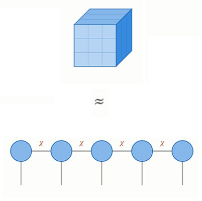
TensorTrainTools provides a compact Tensor Train representation for high-rank tensors, together with the standard operations of the tensor-train toolkit: decomposition of dense arrays with controlled truncation, rank compression, orthogonalization, norms and inner products computed without ever forming the dense tensor, and exact tensor arithmetic through familiar operators. A tensor with millions or billions of entries whose content is structured is often representable by a few thousand parameters. This paclet lets you find that representation, verify its accuracy, and keep computing inside it.

Installation Instructions

To install this paclet in your Wolfram Language environment, evaluate this code:
PacletInstall["RubenRanval/TensorTrainTools"]

To load the code after installation, evaluate this code:
Needs["RubenRanval`TensorTrainTools`"]

Details

A tensor train represents a rank-d tensor as a chain of d rank-3 cores. Storage scales as O(d·n·χ²) in the bond dimension χ instead of O(nᵈ).

Standard operators work directly on tensor trains: t₁+t₂, ct (multiplication by a scalar c), t₁-t₂, and the elementwise product (also known as Hadamard product) t₁⊙ t₂.

Arithmetic is exact and grows bond dimensions (sums add ranks, Hadamard product multiply them). Using TensorTrainCompress allows the reduce bond dimension after each operation.

Applications span high-dimensional PDEs, fluid dynamics, quantum many-body physics (where tensor train are known as matrix product states, MPS), and machine learning for compressing neural network layers.

Paclet Guide

Examples

Basic Examples

Decompose a structured tensor t into a tensor train tt:

In[1]:=

$t = N@Table[Sin[x + y + z], {x, 20}, {y, 20}, {z, 20}]; tt = TensorTrainDecomposition[t, Tolerance -> 10^-10]$

Out[2]=

The compression factor (the ration between the number of stored elements and the number of elements in the dense tensor) can be accessed in the summary box or with the "CompressionRatio" property:

In[3]:=

Out[3]=

The representation is accurate to machine precision:

In[4]:=

Out[4]=

One can visualize the tensor train structure quickly with a tensor network diagram, using the "Diagram" property:

In[5]:=

Out[5]=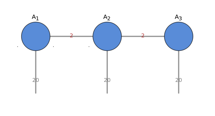

One can then perform arithmetic on tensor trains. Arithmetic stays in the compressed format:

In[6]:=

Out[6]=

In[7]:=

Out[7]=

As we can see, the bond dimensions add up:

In[8]:=

Out[8]=

In[9]:=

Out[9]=

A rank-40 tensor with 2⁴⁰ entries (about 8 TB dense) can be held in a few thousand parameters, with its norm computed directly in the compressed format. Here we are generating a random tensor train representing a tensor of dimensions 2 ⨯ 2 ⨯ … ⨯ 2 with max bond dimensions {2, 4, 4, …, 4, 2}:

In[10]:=

Out[10]=

We can get the full element count of the corresponding dense tensor:

In[11]:=

Out[11]=

We can also get the number of entries actually stored in the cores of the tensor train:

In[12]:=

Out[12]=

And compute the norm directly on the tensor train, without ever generating the full dense tensor:

In[13]:=

Out[13]=

Publisher

Ruben Ranval

Compatibility

Wolfram Language Version 14

External Links

Version History

1.0.0 – 20 July 2026

License Information

MIT License

Paclet Source

Source Metadata

Citation:
- I. V. Oseledets, "Tensor Train Decomposition", SIAM Journal on Scientific Computing 33(5), 2295–2317 (2011), doi:10.1137/090752286
- I. V. Oseledets and E. E. Tyrtyshnikov, "Breaking the curse of dimensionality, or how to use SVD in many dimensions", SIAM J. Sci. Comput. 31(5), 3744–3759 (2009), doi:10.1137/090748330
- U. Schollwöck, "The density-matrix renormalization group in the age of matrix product states", Annals of Physics 326(1), 96–192 (2011)
- I. V. Oseledets and E. E. Tyrtyshnikov, "TT cross-approximation for multidimensional arrays", Linear Algebra and its Applications 432(1), 70–88 (2010)