Basic Examples (2)
Generate an Association to label the results of different operations on an expression:
Perform multiple statistical operations on a single distribution, returning a single expression:
Statistical Examples (11)
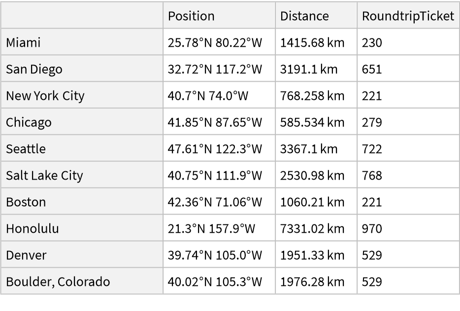
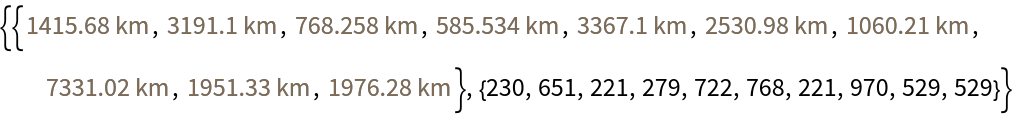
The keys are cities and the values are the cost of a round trip airplane ticket:
I create a function to compute the geographical coordinates of a place from Wikidata:
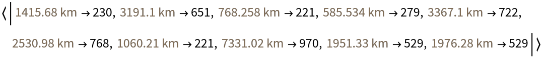
compute the distances to the cities:
organize the data for processing:
turn the data into an association:
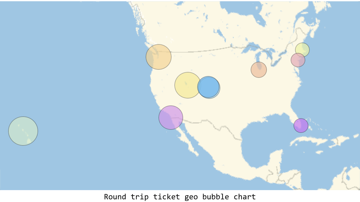
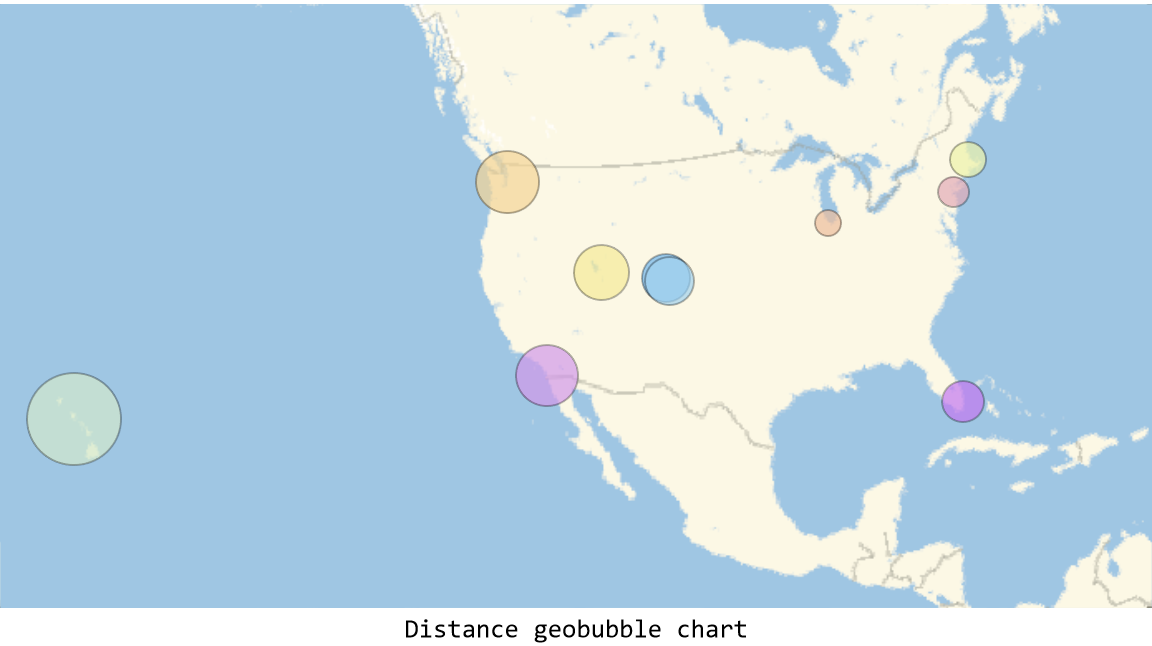
Make a geo bubble chart for the cost of the round trip ticket and the distance:
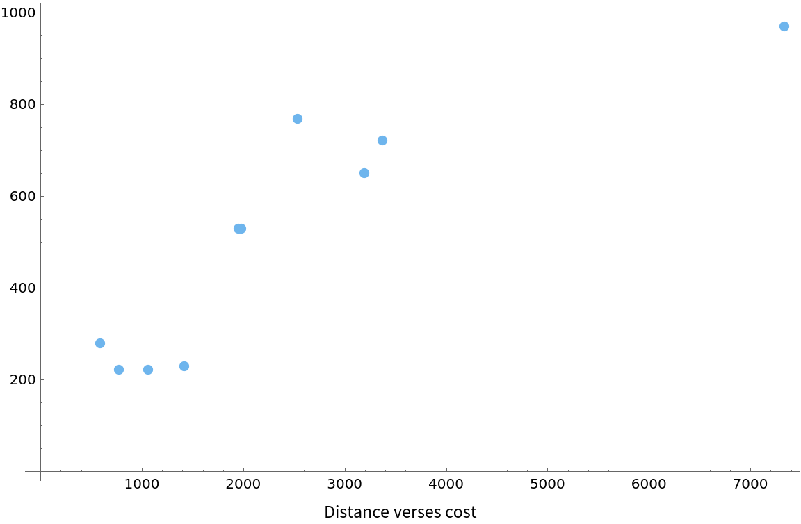
Make a plot of distance and cost:
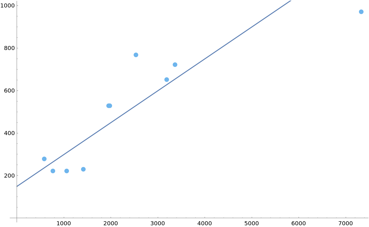
I think the line starts at 100 and has a slope of 0.15:
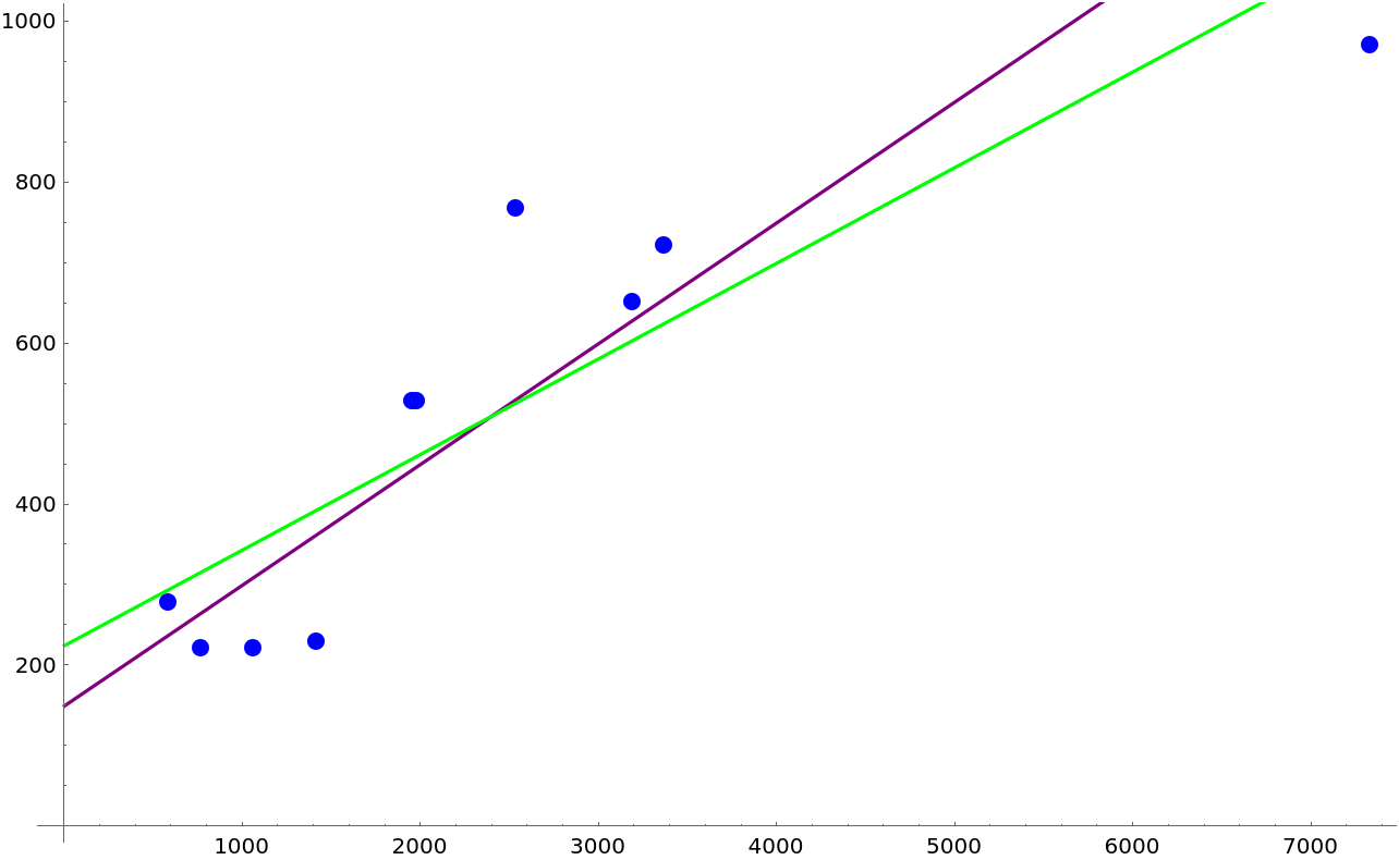
Let's test our prediction with linear interpolation:
Calculate the linear interpolation for the data:
The correct line of best fit is in green and my guess for the line of best fit is in purple:
Neat Examples (8)
Create a constant association:
Partition an association:
Combine partitioning associations with other association operations like AssociationThread:
Create a nested dataset:
Create a large nested association:
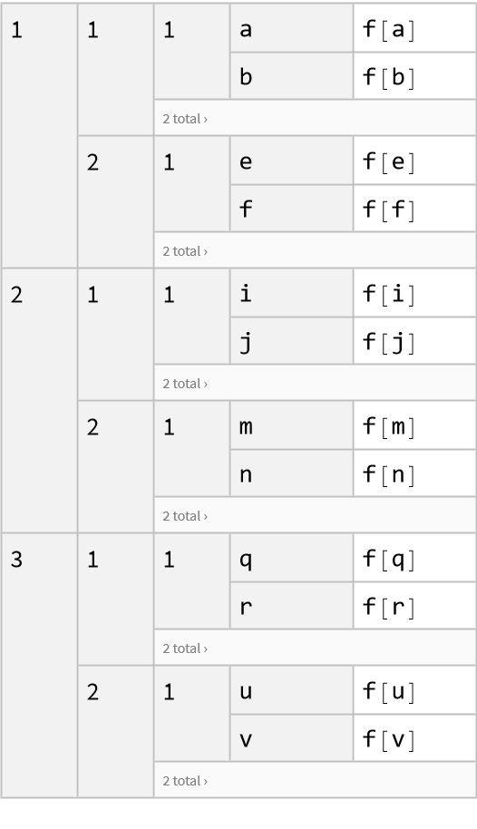
Make a large nested dataset:
Find all the properties for a linear model fit:
Find all the values for a country:

![WikidataGeoPosition[place_?StringQ] := First[WikidataData[First[WikidataSearch[place]], ExternalIdentifier["WikidataID", "P625", <|"Label" -> "coordinate location", "Description" -> "geocoordinates of the subject. For Earth, please note that only WGS84 coordinating system is supported at the moment"|>]]]](https://www.wolframcloud.com/obj/resourcesystem/images/e0a/e0a702b8-7390-472e-b8a7-99a8cd7f5e4a/25b7faf8ab5a948a.png)
![data = AssociationMap[<|"Position" -> WikidataGeoPosition[#], "Distance" -> GeoDistance[Here, WikidataGeoPosition[#]], "RoundtripTicket" -> cities[#]|> &, Keys[cities]]](https://www.wolframcloud.com/obj/resourcesystem/images/e0a/e0a702b8-7390-472e-b8a7-99a8cd7f5e4a/0e95b2ab85b0019f.png)

![Labeled[GeoBubbleChart[
AssociationThread[Values@Normal@dataset[All, "Position"], Values@Normal@dataset[All, "RoundtripTicket"]], Sequence[
ImageSize -> Large, GeoBackground -> "VectorClassic", ChartStyle -> "Pastel"]], "Round trip ticket geo bubble chart"]](https://www.wolframcloud.com/obj/resourcesystem/images/e0a/e0a702b8-7390-472e-b8a7-99a8cd7f5e4a/730950fa48734049.png)
![Labeled[GeoBubbleChart[
AssociationThread[Values@Normal@dataset[All, "Position"], Values@Normal@dataset[All, "Distance"]], Sequence[
ImageSize -> Large, GeoBackground -> "VectorClassic", ChartStyle -> "Pastel"]], "Distance geobubble chart"]](https://www.wolframcloud.com/obj/resourcesystem/images/e0a/e0a702b8-7390-472e-b8a7-99a8cd7f5e4a/7b20ade91eccc9c7.png)
![Labeled[ListPlot[
AssociationThread[Values@Normal@dataset[All, "Distance"], Values@Normal@dataset[All, "RoundtripTicket"]], ImageSize -> Large,
PlotStyle -> "Pastel"], "Distance verses cost"]](https://www.wolframcloud.com/obj/resourcesystem/images/e0a/e0a702b8-7390-472e-b8a7-99a8cd7f5e4a/12405bc42e242355.png)
![Show[ListPlot[
AssociationThread[Values@Normal@dataset[All, "Distance"], Values@Normal@dataset[All, "RoundtripTicket"]], ImageSize -> Full, PlotStyle -> "Pastel"], Plot[150 + 0.15 x, {x, 0, 7000}]]](https://www.wolframcloud.com/obj/resourcesystem/images/e0a/e0a702b8-7390-472e-b8a7-99a8cd7f5e4a/001013e84b0824ce.png)
![CopyToClipboard[
Rasterize@
Show[ListPlot[
AssociationThread[Values@Normal@dataset[All, "Distance"], Values@Normal@dataset[All, "RoundtripTicket"]], ImageSize -> Full, PlotStyle -> "Pastel"], Plot[150 + 0.15 x, {x, 0, 7000}]]]](https://www.wolframcloud.com/obj/resourcesystem/images/e0a/e0a702b8-7390-472e-b8a7-99a8cd7f5e4a/6be68424cfa3e7ed.png)
![linearModelFit = LinearModelFit[
Transpose@{Values@
Normal@dataset[All, QuantityMagnitude[#Distance] &], Values@Normal@dataset[All, #RoundtripTicket &]}, x, x]](https://www.wolframcloud.com/obj/resourcesystem/images/e0a/e0a702b8-7390-472e-b8a7-99a8cd7f5e4a/260615d398906f06.png)
![Show[ListPlot[linearModelFit["Data"], ImageSize -> Full, PlotStyle -> Blue], Plot[150 + 0.15 x, {x, 0, 7000}, PlotStyle -> Purple], Plot[linearModelFit[x], {x, 0, QuantityMagnitude@Max@dataset[All, #Distance &]}, PlotStyle -> Green]]](https://www.wolframcloud.com/obj/resourcesystem/images/e0a/e0a702b8-7390-472e-b8a7-99a8cd7f5e4a/750b8866934e2c58.png)

![AssociationThread[
Range[3] -> (AssociationThread[Range[2] -> #] & /@ Partition[
AssociationThread[Range[2] -> #] & /@ Partition[
AssociationPartition[
AssociationMap[f, ToExpression /@ Alphabet[][[;; 24]]], 2], 2], 2])]](https://www.wolframcloud.com/obj/resourcesystem/images/e0a/e0a702b8-7390-472e-b8a7-99a8cd7f5e4a/416c683f50e37c1e.png)

![AssociationThread[
Range[3] -> (AssociationThread[Range[2] -> #] & /@ Partition[
AssociationThread[Range[2] -> #] & /@ Partition[
AssociationPartition[AssociationMap[f, Array[a, 24]], 2], 2], 2])]](https://www.wolframcloud.com/obj/resourcesystem/images/e0a/e0a702b8-7390-472e-b8a7-99a8cd7f5e4a/1401b5a3b0eda356.png)