Wolfram Language Paclet Repository

Community-contributed installable additions to the Wolfram Language

Primary Navigation

    • Cloud & Deployment
    • Core Language & Structure
    • Data Manipulation & Analysis
    • Engineering Data & Computation
    • External Interfaces & Connections
    • Financial Data & Computation
    • Geographic Data & Computation
    • Geometry
    • Graphs & Networks
    • Higher Mathematical Computation
    • Images
    • Knowledge Representation & Natural Language
    • Machine Learning
    • Notebook Documents & Presentation
    • Scientific and Medical Data & Computation
    • Social, Cultural & Linguistic Data
    • Strings & Text
    • Symbolic & Numeric Computation
    • System Operation & Setup
    • Time-Related Computation
    • User Interface Construction
    • Visualization & Graphics
    • Random Paclet
    • Alphabetical List
  • Using Paclets
    • Get Started
    • Download Definition Notebook
  • Learn More about Wolfram Language

TensorNetworks

Guides

  • TensorNetworks

Tech Notes

  • Building Tensor Networks
  • Contraction Paths and Execution
  • Index conventions and contraction path
  • Matrix Product States
  • A Working Tour of the Symmetry Functions
  • Tensor Networks Overview
  • Young Tableaux and Tensor Symmetries

Symbols

  • ActivateTensors
  • BinaryTensorNetwork
  • BinaryTensorNetworkQ
  • CanonicalPath
  • CanonicalPathQ
  • ContractIndices
  • ContractionTree
  • EinsteinSummation
  • GreedyContractionPath
  • HookFactor
  • HookLength
  • HookLengths
  • IndexedMultiply
  • InitializeTensorNetwork
  • MPSCanonicalForm
  • MPSCanonicalQ
  • MPSEntanglementEntropy
  • MPSNormalize
  • MPSNorm
  • MPSOverlap
  • MPSSchmidtValues
  • MPSTruncate
  • OptimalContractionPath
  • PartitionQ
  • PathIndexContractions
  • PathQ
  • PathToTreePath
  • RandomTensorNetwork
  • SchurDimension
  • SparseTensorNetwork
  • TableauColumns
  • TableauDimension
  • TableauRows
  • TableauShape
  • TableauSize
  • TableauWeylDimension
  • TensorNetworkAdd
  • TensorNetworkContraction
  • TensorNetworkContractions
  • TensorNetworkContract
  • TensorNetworkData
  • TensorNetworkDelete
  • TensorNetworkFreeIndices
  • TensorNetworkGraphData
  • TensorNetworkGraphQ
  • TensorNetworkIndexDimensions
  • TensorNetworkIndexGraph
  • TensorNetworkIndices
  • TensorNetwork
  • TensorNetworkQ
  • TensorNetworkRemoveCycles
  • TensorNetworkReplaceIndices
  • TensorNetworkSize
  • TensorNetworkTensors
  • TensorNetworkToNetGraph
  • ToTensorNetworkGraph
  • TransposePartition
  • TreePathQ
  • TreePathToPath
  • YoungProject
  • YoungSymmetrize
  • YoungTableau
  • YoungTableauQ
  • $TensorNetworkContractionMethods
Index conventions and contraction path
This tech note pins down the index conventions the
Wolfram
TensorNetworks`` kernel uses and shows how the same contraction reads in each one. The conventions look alike (everything is a list of small integers) but they count different things, and conflating them is the usual source of confusion. We work computation-first: every claim below is produced by a cell you can rerun, and we read the meaning off the output rather than asserting it.
Five conventions appear. Four of them number legs, where a leg is a single index of a tensor (one of its axes); one numbers operands, where an operand is a whole tensor taking part in a contraction. The operands are not fixed: at the start they are the input tensors, and each contraction step replaces the two tensors it combines with their single result, so an operand can be an original input or an intermediate produced by an earlier step. Keeping the leg-versus-operand split in mind answers most questions on sight: when you see a list of integer pairs, ask "pairs of what", legs or operands.
Convention
An integer means
A contraction is written as
EinsteinSummation
label
an abstract name
the same name on two tensors
TensorNetwork
data label
a tensor-position, leg-label tag per leg
a bond group (the legs sharing a label)
TensorContract
global slot
a slot in the flattened
TensorProduct
a pair of global slots
ArrayDot
operand-local axis
an axis within one operand
a pair of operand-local axes
contraction-path position
a position in the operand list
a pair of operands to multiply
Three of these four leg conventions give a leg a fixed identity, no matter how the network is contracted; the fourth, the
ArrayDot
operand-local axes, is meaningful only during a contraction step. We build one small network, read its indices in those three fixed conventions, then see how a contraction path (operands) and
ArrayDot
(operand-local axes) re-express the same sums, and close with the two cases a repeated index can take beyond a plain pairwise contraction: broadcasting and hyperedges. Each section re-creates the running network so it stands on its own.
Load tensor network paclet:
In[6]:=
Needs["Wolfram`TensorNetworks`"]
Setup: one small network
We use three tensors in a chain, with
EinsteinSummation
labels
i=1
,
j=2
,
k=3
,
l=4
,
m=5
:
t1
carries
(i,j)
,
t2
carries
(j,k,l)
,
t3
carries
(k,l,m)
. So
j
is a bond between
t1
and
t2
, while
k
and
l
are two bonds between
t2
and
t3
, and
i
(on
t1
) and
m
(on
t3
) are the free legs. We ask for the output in the natural order
(i,m)
. We use symbolic arrays (
ArraySymbol
) so the structural outputs display by name rather than as numbers.
Define the tensors and the network:
In[7]:=
t1=ArraySymbol["t1",{2,3}];t2=ArraySymbol["t2",{3,4,5}];t3=ArraySymbol["t3",{4,5,2}];​​tn=
TensorNetwork
[{t1,t2,t3},{{1,2},{2,3,4},{3,4,5}}{1,5}]
Out[8]=
TensorNetwork
Tensors: 3
Binary: Yes
Free indices: 2
Sparse: No
Output dimension: 4
​

The tensor network is binary: every index sits on at most two tensors, so every contraction is an ordinary pair of tensors. The doubled bond between
t2
and
t3
makes the multi-axis
ArrayDot
case concrete, and the rank-3 tensors make the
TensorContract
blocks nontrivial. As an
EinsteinSummation
string the same network is
"ij,jkl,klm->im"
. The three-or-more case is the subject of the last section.
1. Reading the legs: EinsteinSummation, data labels, global slots
Three of the four leg conventions give a leg a fixed identity, independent of any contraction; we read them off the tensor network here. The fourth, the
ArrayDot
operand-local axes, comes with the contraction in section 3.
EinsteinSummation labels. A label is an abstract name. A label that appears on two tensors is contracted; a label that appears once is free; the part after
->
fixes the output order. That is the entire convention, and
"ij,jkl,klm->im"
already encodes it:
j
,
k
,
l
repeat (contracted),
i
,
m
appear once (free), and the output is the two free legs.
Data labels.
TensorNetworkData
is the low-level form the rest of the kernel consumes. It tags every leg with its tensor position and its label (a
Superscript
of position over label), so a leg is addressable by which tensor and which label. List the per-leg labels:
In[9]:=
tn["Indices"]
Out[9]=
{{
1
1
,
2
1
},{
2
2
,
3
2
,
4
2
},{
3
3
,
4
3
,
5
3
}}
Each entry is one leg, tagged by tensor position (the base) and
EinsteinSummation
label (the superscript); the position-2, label-4 entry, for instance, is tensor 2's
l
-leg. Read off the bonds:
In[10]:=
tn["Bonds"]
Out[10]=
{{
2
1
,
2
2
}3,{
3
2
,
3
3
}4,{
4
2
,
4
3
}5}
This gives the three bond groups with their dimensions: the
j
-bond has dimension 3, the
k
-bond dimension 4, and the
l
-bond dimension 5. Each bond pairs the two legs that share a label and records the dimension summed over it. Now the free legs, the labels that appear on only one tensor:
In[11]:=
tn["FreeIndices"]
Out[11]=
{1,5}
The result is
{1,5}
, the free labels
i,m
in the requested output order. Now tag every leg as either a bond group or a bare free label:
In[12]:=
tn["Contractions"]
Out[12]=
{{
1
1
,{
2
1
,
2
2
}},{{
2
1
,
2
2
},{
3
2
,
3
3
},{
4
2
,
4
3
}},{{
3
2
,
3
3
},{
4
2
,
4
3
},
5
3
}}
The result mirrors the per-tensor shape: the row for
t1
is its free
i
followed by the
j
-bond; the row for
t2
is the
j
-,
k
- and
l
-bonds; the row for
t3
is the
k
-bond, the
l
-bond, then its free
m
. A leg shown as a bare label is free; a leg shown as a list is contracted, and that list names exactly the legs it sums with.
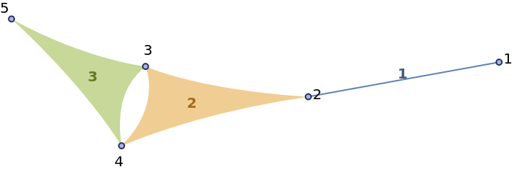
The same bond-versus-free structure is easier to take in as a picture. Draw the network as a hypergraph:
In[7]:=
tn["Hypergraph"]
Out[7]=
In this drawing the vertices are the indices
i,j,k,l,m
and each edge is a tensor, spanning the indices it carries:
t1
over
{i,j}
,
t2
over
{j,k,l}
,
t3
over
{k,l,m}
. An index that lies on two tensors is a contracted bond, that is, a vertex shared by two edges:
j
joins
t1
and
t2
, while
k
and
l
both join
t2
and
t3
(the doubled bond). An index on a single tensor is free, a vertex in just one edge:
i
on
t1
and
m
on
t3
. This is the same split that the contractions listing gave, now visible at a glance. Note it is the dual of the usual tensor-network diagram, where tensors are nodes and indices are lines; here the two roles are swapped.
Global slots. Contraction flattens the operands into one
TensorProduct
, and a global index is a slot position in that flattened product. Lower the
EinsteinSummation
spec to see those slots:
In[13]:=
EinsteinSummation
["ij,jkl,klm->im",{t1,t2,t3}]
Out[13]=
TensorContract
2
t1

3
t2

3
t3
,{{2,3},{4,6},{5,7}}
The output is an inactive
TensorContract
of the
TensorProduct
with contraction pairs
{{2,3},{4,6},{5,7}}
. The integers are slot positions in the flattened
TensorProduct[t1,t2,t3]
. To see the slots explicitly, flatten the data labels:
In[14]:=
Catenate[tn["Indices"]]
Out[14]=
{
1
1
,
2
1
,
2
2
,
3
2
,
4
2
,
3
3
,
4
3
,
5
3
}
The result lists the eight legs in order, and the
n
-th element is global slot
n
: its base is the tensor, its superscript the
EinsteinSummation
label. So
t1
owns slots 1-2,
t2
owns 3-5,
t3
owns 6-8, and the lowering reads: sum slot 2 with 3 (the two
j
's), 4 with 6 (
k
), 5 with 7 (
l
). The free slots 1 (
i
) and 8 (
m
) survive in slot order
(i,m)
, which is the order we requested, so there is no trailing transpose. Output order is its own convention: free legs survive tensor-then-leg, and requesting a different order would append a
Transpose
.
2. The contraction-path convention: pairwise steps over operands
Contraction happens pairwise and in sequence. A path is a list of steps; each step picks two tensors from the current pool, sums over every leg they share, and puts the resulting tensor back in the pool for the later steps. The path numbers operands, not legs: it says which two tensors meet at each step, and the legs that get summed are simply whatever those two share. The final value does not depend on the order, but the order is what the executor walks, and it fixes which indices are summed when.
Get a contraction path for the tensor network and keep it:
In[15]:=
path=
GreedyContractionPath
[tn]
Out[15]=
{{2,3},{1,2}}
The result
{{2,3},{1,2}}
is two steps over the three operands
{t1,t2,t3}
. Step 1's
{2,3}
contracts operands 2 and 3 (
t2
,
t3
); their result re-enters the pool, now
{t1,t2t3}
, so step 2's
{1,2}
means
t1
and
t2t3
. Operand numbers are reused because after each contraction the two inputs are replaced by their single result. (
GreedyContractionPath
is one of several functions that compute such a path; they differ in the cost of the path they return, not in any index convention, so we just use one.)
The path is an abstract recipe; the executor turns it into an explicit nest of pairwise contractions. Build that expression, left inactive so we can read the plan:
In[16]:=
ic=
TensorNetworkContraction
[tn,path]
Out[16]=
ArrayDot
2
t1
,ArrayDot
3
t2
,
3
t3
,{{2,1},{3,2}},{{2,1}}
The output is
ArrayDot[t1,ArrayDot[t2,t3,{{2,1},{3,2}}],{{2,1}}]
(inactive), read inside-out. The inner
ArrayDot
is step 1: contract
t2
and
t3
over their two shared legs
k,l
(the operand-local axis pairs
{{2,1},{3,2}}
of section 3). The outer
ArrayDot
is step 2: contract
t1
with that intermediate over their shared
j
. The nesting is the order, and each node carries the axes summed at that step.
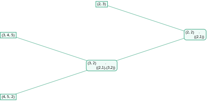
The same thing is clearer as a tree. Render the contraction hierarchy with dimension labels:
In[17]:=
ContractionTree
[ic,"Labels""Dimensions"]
Out[17]=
The leaves are the input tensors (dims
{2,3}
,
{3,4,5}
,
{4,5,2}
), and each internal node is one pairwise contraction, annotated by the axes it sums and the dimensions of its result. The lower node contracts
t2
with
t3
over
{{2,1},{3,2}}
to make a
{3,2}
tensor (legs
j,m
); the root contracts
t1
with that over
{{2,1}}
to make the final
{2,2}
(legs
i,m
). Reading the tree bottom-up gives the exact contraction sequence, and reading a node tells you which legs were summed there.
In words, the sequence is: start with
t1
(i,j)
,
t2
(j,k,l)
,
t3
(k,l,m)
; step 1 sums the two shared legs
k,l
to get the intermediate
(j,m)
; step 2 sums the shared
j
to get
(i,m)
. Every step sums exactly the legs common to the two operands it joins, and the free legs of both survive into the result.
The path itself never mentions
j,k,l
; the summed legs are implied by which operands meet. Recover them explicitly:
In[18]:=
PathIndexContractions
path,
TensorNetworkData
[tn]
Out[18]=
{{4,6},{5,7},{2,3}}
The output
{{4,6},{5,7},{2,3}}
lists the summed legs as global slots, one step at a time: step 1 sums slots
{4,6}
(
k
) and
{5,7}
(
l
), step 2 sums
{2,3}
(
j
). Those are exactly the lowering pairs from section 1, regrouped by path step, the bridge from the operand-only path back to the leg conventions.
Finally, the operand numbering has an alternative that never reuses a number, giving every tensor and intermediate a permanent id. Request it:
In[19]:=
GreedyContractionPath
[tn,"FixedIndexing"True]
Out[19]=
{{2,3},{4,1}}
The same tree now reads
{{2,3},{4,1}}
: merging operands 2 and 3 creates the intermediate with id 4, and step 2 joins operand 1 with that stable 4. Same sequence, two operand-numbering conventions.
3. The ArrayDot convention: operand-local axes
The executor contracts two tensors at a time, and its default primitive
ArrayDot
uses the fourth leg convention: it names each operand's own axes. A contraction is a list of
{axisInA,axisInB}
pairs, each axis counted within its own tensor. The doubled bond between
t2
and
t3
(the shared legs
k,l
) makes this concrete. Instantiate the two tensors numerically (call the instances
b
and
c
) and contract over
k,l
three equivalent ways:
In[20]:=
With[{b=RandomReal[1,{3,4,5}],c=RandomReal[1,{4,5,2}]},​​ArrayDot[b,c,{{2,1},{3,2}}]​​ArrayDot[b,c,2]​​TensorContract[TensorProduct[b,c],{{2,4},{3,5}}]]
Out[20]=
True
The result is
True
, so all three name the same contraction. The first is the
ArrayDot
pair form:
{2,1}
contracts
t2
's axis 2 (
k
) with
t3
's axis 1 (
k
),
{3,2}
contracts
t2
's axis 3 (
l
) with
t3
's axis 2 (
l
). The second is the count form
ArrayDot[b,c,2]
, which contracts
t2
's last two axes with
t3
's first two; it works here only because the shared axes happen to be
t2
's trailing block and
t3
's leading block. The third is the global-slot form, and comparing it to the pair form gives the translation: an
a
-axis keeps its number, while
b
's axis
bi
is the global slot
rank[a]+bi
(here
rank[t2]=3
, so
t3
's axes 1,2 are global slots 4,5). The point of the operand-local convention is that a pairwise step never builds the growing flattened slot list; it only ever names two operands' own axes, which is why
ArrayDot
is the cheap default.
4. The same contraction in every convention
Putting it together, here is the single sum over
j
(the bond between
t1
and
t2
) in all five conventions:
Convention
the sum over
j
EinsteinSummation
the repeated label
j
in
"ij,jkl,klm->im"
TensorNetwork
data
the bond group joining
t1
's
j
-leg and
t2
's
j
-leg
TensorContract
global slots
the pair
{2,3}
(slot 2 is
t1
's
j
, slot 3 is
t2
's
j
)
ArrayDot
operand-local
{2,1}
(axis 2 of
t1
with axis 1 of
t2
)
contraction path
implicit in the step that contracts the operands holding
t1
and
t2
The translations are mechanical: lay all legs end to end and a repeated
EinsteinSummation
label becomes the pair of its two global slots; a
b
-axis at global slot
s
is operand-local axis
s-rank[a]
(here
t2
's
j
at slot 3 is local axis
3-2=1
); a path step names two operands and the summed legs are the labels they share.
5. What else a repeated index can mean
A repeated index in the tensor network is always a plain pairwise contraction. Two other cases exist, and each has its own index convention.
Lower the four-tensor network:
The contraction-path machinery cannot use a three-way group, because a path is built from pairwise steps. It instead binarizes: it inserts an explicit delta "spider" tensor so the hyperedge becomes ordinary two-tensor bonds. Build the four-tensor network:
As one can see the index/leg 3 is shared by three tensors:
Its binarized form adds one spider, raising the operand count from four to five:
The greedy path then runs over that five-operand pool:
Where this leaves us
We built one network and read its indices in every convention the kernel uses:

© 2026 Wolfram. All rights reserved.

  • Legal & Privacy Policy
  • Contact Us
  • WolframAlpha.com
  • WolframCloud.com