Wolfram Language
Paclet Repository
Community-contributed installable additions to the Wolfram Language
Primary Navigation
Categories
Cloud & Deployment
Core Language & Structure
Data Manipulation & Analysis
Engineering Data & Computation
External Interfaces & Connections
Financial Data & Computation
Geographic Data & Computation
Geometry
Graphs & Networks
Higher Mathematical Computation
Images
Knowledge Representation & Natural Language
Machine Learning
Notebook Documents & Presentation
Scientific and Medical Data & Computation
Social, Cultural & Linguistic Data
Strings & Text
Symbolic & Numeric Computation
System Operation & Setup
Time-Related Computation
User Interface Construction
Visualization & Graphics
Random Paclet
Alphabetical List
Using Paclets
Create a Paclet
Get Started
Download Definition Notebook
Learn More about
Wolfram Language
QuantileRegression
Guides
Quantile regression
Tech Notes
Quantile regression 3D examples
Quantile regression over weather time series
Symbols
NURBSBasis
QuantileEnvelope
QuantileEnvelopeRegion
QuantileRegressionFit
QuantileRegression
Quantile regression over weather time series
I
n
t
r
o
d
u
c
t
i
o
n
E
s
t
i
m
a
t
i
o
n
o
f
c
o
n
d
i
t
i
o
n
a
l
d
e
n
s
i
t
y
d
i
s
t
r
i
b
u
t
i
o
n
s
Q
u
a
n
t
i
l
e
r
e
g
r
e
s
s
i
o
n
o
v
e
r
h
e
t
e
r
o
s
c
e
d
a
s
t
i
c
d
a
t
a
Introduction
In this notebook we show two primary use cases of for Quantile Regression (QR):
◼
Fitting regression quantiles over
h
e
t
e
r
o
s
c
e
d
a
s
t
i
c
d
a
t
a
◼
Estimation of conditional density
distributions
Quantile regression over heteroscedastic data
Load the paclet
I
n
[
2
4
2
]
:
=
N
e
e
d
s
[
"
A
n
t
o
n
A
n
t
o
n
o
v
`
Q
u
a
n
t
i
l
e
R
e
g
r
e
s
s
i
o
n
`
"
]
Take temperature data
I
n
[
2
4
3
]
:
=
t
s
T
e
m
p
=
W
e
a
t
h
e
r
D
a
t
a
[
{
"
A
t
l
a
n
t
a
"
,
"
G
e
o
r
g
i
a
"
}
,
"
T
e
m
p
e
r
a
t
u
r
e
"
,
{
{
2
0
1
8
,
1
,
1
}
,
{
2
0
2
3
,
1
,
1
}
,
"
D
a
y
"
}
]
O
u
t
[
2
4
3
]
=
T
i
m
e
S
e
r
i
e
s
T
i
m
e
:
0
1
J
a
n
2
0
1
8
G
M
T
-
4
t
o
0
1
J
a
n
2
0
2
3
G
M
T
-
4
D
a
t
a
p
o
i
n
t
s
:
1
8
2
7
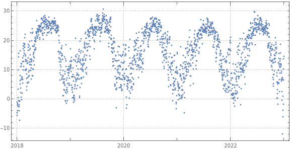
Plot time series points
I
n
[
2
4
4
]
:
=
o
p
t
s
=
{
I
m
a
g
e
S
i
z
e
L
a
r
g
e
,
A
s
p
e
c
t
R
a
t
i
o
1
/
2
,
P
l
o
t
T
h
e
m
e
"
D
e
t
a
i
l
e
d
"
,
J
o
i
n
e
d
F
a
l
s
e
}
;
D
a
t
e
L
i
s
t
P
l
o
t
[
t
s
T
e
m
p
,
o
p
t
s
]
O
u
t
[
2
4
4
]
=
Data summary
I
n
[
2
4
5
]
:
=
R
e
s
o
u
r
c
e
F
u
n
c
t
i
o
n
[
"
R
e
c
o
r
d
s
S
u
m
m
a
r
y
"
]
[
t
s
T
e
m
p
[
"
P
a
t
h
"
]
]
O
u
t
[
2
4
5
]
=
1
c
o
l
u
m
n
1
M
i
n
3
.
7
2
3
7
5
×
9
1
0
1
s
t
Q
u
3
.
7
6
3
1
7
×
9
1
0
M
e
a
n
3
.
8
0
2
6
4
×
9
1
0
M
e
d
i
a
n
3
.
8
0
2
6
4
×
9
1
0
3
r
d
Q
u
3
.
8
4
2
1
×
9
1
0
M
a
x
3
.
8
8
1
5
2
×
9
1
0
,
2
c
o
l
u
m
n
2
2
3
.
8
9
°
C
1
6
2
4
.
2
2
°
C
1
6
1
2
.
7
8
°
C
1
4
2
2
.
7
8
°
C
1
2
2
5
°
C
1
2
2
3
.
3
3
°
C
1
1
(
O
t
h
e
r
)
1
7
4
6
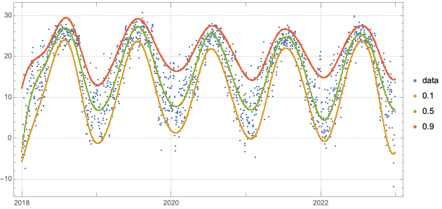
Find regression quantiles for 0.1, 0.5, 0.9
I
n
[
2
4
6
]
:
=
A
b
s
o
l
u
t
e
T
i
m
i
n
g
p
r
o
b
s
=
{
0
.
1
,
0
.
5
,
0
.
9
}
;
q
F
u
n
c
s
=
Q
u
a
n
t
i
l
e
R
e
g
r
e
s
s
i
o
n
[
Q
u
a
n
t
i
t
y
M
a
g
n
i
t
u
d
e
[
t
s
T
e
m
p
[
"
P
a
t
h
"
]
]
,
1
6
,
p
r
o
b
s
]
;
O
u
t
[
2
4
6
]
=
{
0
.
9
5
3
4
0
9
,
N
u
l
l
}
Plot time series points with fitted regression quantiles
I
n
[
2
4
7
]
:
=
D
a
t
e
L
i
s
t
P
l
o
t
[
{
t
s
T
e
m
p
[
"
P
a
t
h
"
]
,
M
a
p
[
F
u
n
c
t
i
o
n
[
{
f
}
,
{
#
,
f
[
#
]
}
&
/
@
t
s
T
e
m
p
[
"
T
i
m
e
s
"
]
]
,
q
F
u
n
c
s
]
}
,
o
p
t
s
,
J
o
i
n
e
d
{
F
a
l
s
e
,
T
r
u
e
,
T
r
u
e
,
T
r
u
e
}
,
P
l
o
t
L
e
g
e
n
d
s
{
"
d
a
t
a
"
,
S
e
q
u
e
n
c
e
@
@
p
r
o
b
s
}
]
O
u
t
[
2
4
7
]
=
Remark:
It should be obvious from the plot above that the time series data is heteroscedastic.
Count the number points under each surface
I
n
[
2
4
8
]
:
=
s
e
p
P
o
i
n
t
s
=
A
s
s
o
c
i
a
t
i
o
n
@
M
a
p
T
h
r
e
a
d
[
F
u
n
c
t
i
o
n
[
{
p
,
f
}
,
p
L
e
n
g
t
h
[
S
e
l
e
c
t
[
Q
u
a
n
t
i
t
y
M
a
g
n
i
t
u
d
e
[
t
s
T
e
m
p
[
"
P
a
t
h
"
]
]
,
#
〚
2
〛
<
f
[
#
〚
1
〛
]
&
]
]
]
,
{
p
r
o
b
s
,
q
F
u
n
c
s
}
]
O
u
t
[
2
4
8
]
=
0
.
1
1
8
2
,
0
.
5
9
1
5
,
0
.
9
1
6
4
7
Show the corresponding fractions (should correspond to the probabilities)
I
n
[
2
4
9
]
:
=
s
e
p
F
r
a
c
t
i
o
n
s
=
N
[
s
e
p
P
o
i
n
t
s
/
L
e
n
g
t
h
[
t
s
T
e
m
p
[
"
P
a
t
h
"
]
]
]
O
u
t
[
2
4
9
]
=
0
.
1
0
.
0
9
9
6
1
6
9
,
0
.
5
0
.
5
0
0
8
2
1
,
0
.
9
0
.
9
0
1
4
7
8
Estimation of conditional density
distributions
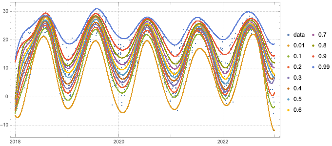
Find regression quantiles for a "comprehensive" set of probabilities
I
n
[
2
5
0
]
:
=
A
b
s
o
l
u
t
e
T
i
m
i
n
g
p
r
o
b
s
=
S
o
r
t
[
J
o
i
n
[
R
a
n
g
e
[
0
.
1
,
0
.
9
,
0
.
1
]
,
{
0
.
0
1
,
0
.
9
9
}
]
]
;
q
F
u
n
c
s
=
Q
u
a
n
t
i
l
e
R
e
g
r
e
s
s
i
o
n
[
Q
u
a
n
t
i
t
y
M
a
g
n
i
t
u
d
e
[
t
s
T
e
m
p
[
"
P
a
t
h
"
]
]
,
1
6
,
p
r
o
b
s
]
;
O
u
t
[
2
5
0
]
=
{
2
.
3
7
6
7
9
,
N
u
l
l
}
Plot time series points with fitted regression quantiles
I
n
[
2
5
1
]
:
=
D
a
t
e
L
i
s
t
P
l
o
t
[
{
t
s
T
e
m
p
[
"
P
a
t
h
"
]
,
M
a
p
[
F
u
n
c
t
i
o
n
[
{
f
}
,
{
#
,
f
[
#
]
}
&
/
@
t
s
T
e
m
p
[
"
T
i
m
e
s
"
]
]
,
q
F
u
n
c
s
]
}
,
o
p
t
s
,
J
o
i
n
e
d
{
F
a
l
s
e
,
T
r
u
e
,
T
r
u
e
,
T
r
u
e
}
,
P
l
o
t
L
e
g
e
n
d
s
{
"
d
a
t
a
"
,
S
e
q
u
e
n
c
e
@
@
p
r
o
b
s
}
]
O
u
t
[
2
5
1
]
=
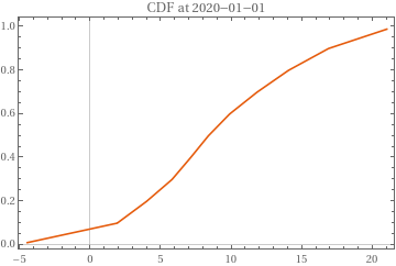
Reconstruct the CDF distribution at the focus point (January 1st, 2020)
I
n
[
2
5
2
]
:
=
f
o
c
u
s
P
o
i
n
t
=
A
b
s
o
l
u
t
e
T
i
m
e
[
{
2
0
2
0
,
1
,
1
}
]
;
x
s
=
T
h
r
o
u
g
h
[
q
F
u
n
c
s
[
f
o
c
u
s
P
o
i
n
t
]
]
;
c
d
f
P
a
i
r
s
=
T
r
a
n
s
p
o
s
e
[
{
x
s
,
p
r
o
b
s
}
]
;
Plot the empirical CDF
I
n
[
2
5
5
]
:
=
L
i
s
t
L
i
n
e
P
l
o
t
c
d
f
P
a
i
r
s
,
O
u
t
[
2
5
5
]
=
In order to plot the corresponding PDF function define a CDF reconstruction function
Plot empirical PDF