Model (6) 

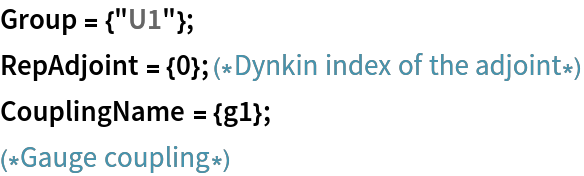
We consider a simple model with a U(1) gauge group. The adjoint representation is trivial for abelian groups and has Dynkin index {0}. We also include a single complex scalar in the fundamental representation (R= 1).

In[1]:=

One complex scalar (interpreted as a Higgs-like field) is present:

In[2]:=

Fermions are treated as Weyl spinors in DRalgo. Therefore, to define a Dirac fermion, one must include both a left-handed and a right-handed Weyl spinor. In this minimal model, no fermions are included:

In[3]:=

We allocate all necessary coupling tensors for the model:

In[4]:=

To build the Lagrangian, we construct the mass term m² ϕ^†ϕ :

In[5]:=

We add the quartic interaction of the complex scalar:

In[6]:=

To invoke the model in DRalgo, it needs to be imported:

In[7]:=

Dimensional reduction from hard to soft scale (9) 

Integrating out the hard-scale modes in verbose mode:

In[8]:=

After the reduction completes, the effective couplings are given by:

In[9]:=

Out[9]=

Internally, a list of constants is used and they can be printed via:

In[10]:=

Out[10]=

Both the leading order (LO) and next-to-leading order (NLO) scalar masses are given by:

In[11]:=

Out[11]=

Out[12]=

Similarly, the Debye masses are given by:

In[13]:=

Out[13]=

Out[14]=

Often one needs the explicit coupling tensors of DRalgo whose indices can be accessed via:

In[15]:=

For a specific tensor, e.g. for the scalars quartics with index "1", we can print it directly:

In[16]:=

Out[16]=

The hard-scale pressure contribution in the high-temperature expansion is obtained by:

In[17]:=

Out[17]=

In[18]:=

Out[18]=

In[19]:=

Out[19]=

Finally, the β-functions of the model are:

In[20]:=

Out[20]=

Dimensional reduction from hard to ''ultrasoft'' scale (6) 

Integrate out the soft-scale modes in verbose mode:

In[21]:=

After the reduction completes, the effective couplings are given by:

In[22]:=

Out[22]=

Both the leading order (LO) and next-to-leading order (NLO) scalar masses are given by:

In[23]:=

Out[23]=

Out[24]=

The soft-scale pressure contribution in the high-temperature expansion is obtained by:

In[25]:=

Out[25]=

In[26]:=

Out[26]=

The NNLO soft-scale pressure is not yet included in DRalgo:

In[27]:=

Finally, the β-functions of the model are:

In[28]:=

Out[28]=

Effective potential directly (3) 

First, the theory scale is chosen:

In[29]:=

Then, a constant background is introduced to the scalars and the potential is calculated:

In[30]:=

Finally, the different orders of the potential can be computed:

In[31]:=

Out[31]=

In[32]:=

Out[32]=

In[33]:=

Out[33]=

Effective potential directly using HEFT (5) 

In this example, we assume that the temporal and vector degrees of freedom are heavy compared to the scalar sector. Thus, we integrate them out starting from the soft theory, ultimately constructing a High-Energy Effective Theory (HEFT).

Start from the soft theory:

In[34]:=

We introduce a background field, φ, for the scalars and calculate the effective potential:

In[35]:=

Before computing the final potential, we must identify which temporal scalars and gauge bosons are heavy and are to be integrated out. Use PrepareHET[{scalarIndices}, {vectorIndices}] to specify them:

In[36]:=

This functions similar to PerformDRsoft[{}], and the indices can be found with the commands

In[37]:=

Out[37]=

Out[38]=

After, calculating the effective potential in the HEFT setup,

In[39]:=

finally, the different orders of the potential can be computed :

In[40]:=

Out[40]=

In[41]:=

Out[41]=

The U(1) gauge bosons modify the scalar kinetic terms. The renormalization (wavefunction normalization) is encoded in the Z-factor:

In[42]:=

Out[42]=