Wolfram Language Paclet Repository
Community-contributed installable additions to the Wolfram Language
Create simple, discrete coils using current-carrying loops, saddles or ellipses to generate magnetic fields
Contributed by: Noah Hardwicke, Peter J. Hobson, Michael Packer
Create simple coils made from cylindrical loop, saddle, or ellipse-based primitives, optimised to generate a target magnetic field harmonic. Visualise and examine the coils and the magnetic fields they generate.
CreateCoil implements the theoretical model derived in Designing optimal loop, saddle, and ellipse-based magnetic coils by spherical harmonic mapping.
We will soon be adding the ability to export coil data and field data, so check back for updates!

To install this paclet in your Wolfram Language environment,
evaluate this code:
PacletInstall["NoahH/CreateCoil"]
To load the code after installation, evaluate this code:
Needs["NoahH`CreateCoil`"]
Compare the uniform axial Bz field (encoded as the B1, 0 field harmonic) generated by a Helmholtz pair, and by three optimised pairs of loops covering the same axial extent:
| In[1]:= | ![{solHelm, sol3Pairs} = First /@ {InterpretationBox[FrameBox[TagBox[TooltipBox[PaneBox[GridBox[List[List[GraphicsBox[List[Thickness[0.0025`], List[FaceForm[List[RGBColor[0.9607843137254902`, 0.5058823529411764`, 0.19607843137254902`], Opacity[1.`]]], FilledCurveBox[List[List[List[0, 2, 0], List[0, 1, 0], List[0, 1, 0], List[0, 1, 0], List[0, 1, 0]], List[List[0, 2, 0], List[0, 1, 0], List[0, 1, 0], List[0, 1, 0], List[0, 1, 0]], List[List[0, 2, 0], List[0, 1, 0], List[0, 1, 0], List[0, 1, 0], List[0, 1, 0], List[0, 1, 0]], List[List[0, 2, 0], List[1, 3, 3], List[0, 1, 0], List[1, 3, 3], List[0, 1, 0], List[1, 3, 3], List[0, 1, 0], List[1, 3, 3], List[1, 3, 3], List[0, 1, 0], List[1, 3, 3], List[0, 1, 0], List[1, 3, 3]]], List[List[List[205.`, 22.863691329956055`], List[205.`, 212.31669425964355`], List[246.01799774169922`, 235.99870109558105`], List[369.0710144042969`, 307.0436840057373`], List[369.0710144042969`, 117.59068870544434`], List[205.`, 22.863691329956055`]], List[List[30.928985595703125`, 307.0436840057373`], List[153.98200225830078`, 235.99870109558105`], List[195.`, 212.31669425964355`], List[195.`, 22.863691329956055`], List[30.928985595703125`, 117.59068870544434`], List[30.928985595703125`, 307.0436840057373`]], List[List[200.`, 410.42970085144043`], List[364.0710144042969`, 315.7036876678467`], List[241.01799774169922`, 244.65868949890137`], List[200.`, 220.97669792175293`], List[158.98200225830078`, 244.65868949890137`], List[35.928985595703125`, 315.7036876678467`], List[200.`, 410.42970085144043`]], List[List[376.5710144042969`, 320.03370475769043`], List[202.5`, 420.53370475769043`], List[200.95300006866455`, 421.42667961120605`], List[199.04699993133545`, 421.42667961120605`], List[197.5`, 420.53370475769043`], List[23.428985595703125`, 320.03370475769043`], List[21.882003784179688`, 319.1406993865967`], List[20.928985595703125`, 317.4896984100342`], List[20.928985595703125`, 315.7036876678467`], List[20.928985595703125`, 114.70369529724121`], List[20.928985595703125`, 112.91769218444824`], List[21.882003784179688`, 111.26669120788574`], List[23.428985595703125`, 110.37369346618652`], List[197.5`, 9.87369155883789`], List[198.27300024032593`, 9.426692008972168`], List[199.13700008392334`, 9.203690528869629`], List[200.`, 9.203690528869629`], List[200.86299991607666`, 9.203690528869629`], List[201.72699999809265`, 9.426692008972168`], List[202.5`, 9.87369155883789`], List[376.5710144042969`, 110.37369346618652`], List[378.1179962158203`, 111.26669120788574`], List[379.0710144042969`, 112.91769218444824`], List[379.0710144042969`, 114.70369529724121`], List[379.0710144042969`, 315.7036876678467`], List[379.0710144042969`, 317.4896984100342`], List[378.1179962158203`, 319.1406993865967`], List[376.5710144042969`, 320.03370475769043`]]]]], List[FaceForm[List[RGBColor[0.5529411764705883`, 0.6745098039215687`, 0.8117647058823529`], Opacity[1.`]]], FilledCurveBox[List[List[List[0, 2, 0], List[0, 1, 0], List[0, 1, 0], List[0, 1, 0]]], List[List[List[44.92900085449219`, 282.59088134765625`], List[181.00001525878906`, 204.0298843383789`], List[181.00001525878906`, 46.90887451171875`], List[44.92900085449219`, 125.46986389160156`], List[44.92900085449219`, 282.59088134765625`]]]]], List[FaceForm[List[RGBColor[0.6627450980392157`, 0.803921568627451`, 0.5686274509803921`], Opacity[1.`]]], FilledCurveBox[List[List[List[0, 2, 0], List[0, 1, 0], List[0, 1, 0], List[0, 1, 0]]], List[List[List[355.0710144042969`, 282.59088134765625`], List[355.0710144042969`, 125.46986389160156`], List[219.`, 46.90887451171875`], List[219.`, 204.0298843383789`], List[355.0710144042969`, 282.59088134765625`]]]]], List[FaceForm[List[RGBColor[0.6901960784313725`, 0.5882352941176471`, 0.8117647058823529`], Opacity[1.`]]], FilledCurveBox[List[List[List[0, 2, 0], List[0, 1, 0], List[0, 1, 0], List[0, 1, 0]]], List[List[List[200.`, 394.0606994628906`], List[336.0710144042969`, 315.4997024536133`], List[200.`, 236.93968200683594`], List[63.928985595703125`, 315.4997024536133`], List[200.`, 394.0606994628906`]]]]]], List[Rule[BaselinePosition, Scaled[0.15`]], Rule[ImageSize, 10], Rule[ImageSize, 15]]], StyleBox[RowBox[List["FindLoopCoil", " "]], Rule[ShowAutoStyles, False], Rule[ShowStringCharacters, False], Rule[FontSize, Times[0.9`, Inherited]], Rule[FontColor, GrayLevel[0.1`]]]]], Rule[GridBoxSpacings, List[Rule["Columns", List[List[0.25`]]]]]], Rule[Alignment, List[Left, Baseline]], Rule[BaselinePosition, Baseline], Rule[FrameMargins, List[List[3, 0], List[0, 0]]], Rule[BaseStyle, List[Rule[LineSpacing, List[0, 0]], Rule[LineBreakWithin, False]]]], RowBox[List["PacletSymbol", "[", RowBox[List["\"NoahH/CreateCoil\"", ",", "\"NoahH`CreateCoil`FindLoopCoil\""]], "]"]], Rule[TooltipStyle, List[Rule[ShowAutoStyles, True], Rule[ShowStringCharacters, True]]]], Function[Annotation[Slot[1], Style[Defer[PacletSymbol["NoahH/CreateCoil", "NoahH`CreateCoil`FindLoopCoil"]], Rule[ShowStringCharacters, True]], "Tooltip"]]], Rule[Background, RGBColor[0.968`, 0.976`, 0.984`]], Rule[BaselinePosition, Baseline], Rule[DefaultBaseStyle, List[]], Rule[FrameMargins, List[List[0, 0], List[1, 1]]], Rule[FrameStyle, RGBColor[0.831`, 0.847`, 0.85`]], Rule[RoundingRadius, 4]], PacletSymbol["NoahH/CreateCoil", "NoahH`CreateCoil`FindLoopCoil"], Rule[Selectable, False], Rule[SelectWithContents, True], Rule[BoxID, "PacletSymbolBox"]][{1}, 1, {0.01, 1}], InterpretationBox[FrameBox[TagBox[TooltipBox[PaneBox[GridBox[List[List[GraphicsBox[List[Thickness[0.0025`], List[FaceForm[List[RGBColor[0.9607843137254902`, 0.5058823529411764`, 0.19607843137254902`], Opacity[1.`]]], FilledCurveBox[List[List[List[0, 2, 0], List[0, 1, 0], List[0, 1, 0], List[0, 1, 0], List[0, 1, 0]], List[List[0, 2, 0], List[0, 1, 0], List[0, 1, 0], List[0, 1, 0], List[0, 1, 0]], List[List[0, 2, 0], List[0, 1, 0], List[0, 1, 0], List[0, 1, 0], List[0, 1, 0], List[0, 1, 0]], List[List[0, 2, 0], List[1, 3, 3], List[0, 1, 0], List[1, 3, 3], List[0, 1, 0], List[1, 3, 3], List[0, 1, 0], List[1, 3, 3], List[1, 3, 3], List[0, 1, 0], List[1, 3, 3], List[0, 1, 0], List[1, 3, 3]]], List[List[List[205.`, 22.863691329956055`], List[205.`, 212.31669425964355`], List[246.01799774169922`, 235.99870109558105`], List[369.0710144042969`, 307.0436840057373`], List[369.0710144042969`, 117.59068870544434`], List[205.`, 22.863691329956055`]], List[List[30.928985595703125`, 307.0436840057373`], List[153.98200225830078`, 235.99870109558105`], List[195.`, 212.31669425964355`], List[195.`, 22.863691329956055`], List[30.928985595703125`, 117.59068870544434`], List[30.928985595703125`, 307.0436840057373`]], List[List[200.`, 410.42970085144043`], List[364.0710144042969`, 315.7036876678467`], List[241.01799774169922`, 244.65868949890137`], List[200.`, 220.97669792175293`], List[158.98200225830078`, 244.65868949890137`], List[35.928985595703125`, 315.7036876678467`], List[200.`, 410.42970085144043`]], List[List[376.5710144042969`, 320.03370475769043`], List[202.5`, 420.53370475769043`], List[200.95300006866455`, 421.42667961120605`], List[199.04699993133545`, 421.42667961120605`], List[197.5`, 420.53370475769043`], List[23.428985595703125`, 320.03370475769043`], List[21.882003784179688`, 319.1406993865967`], List[20.928985595703125`, 317.4896984100342`], List[20.928985595703125`, 315.7036876678467`], List[20.928985595703125`, 114.70369529724121`], List[20.928985595703125`, 112.91769218444824`], List[21.882003784179688`, 111.26669120788574`], List[23.428985595703125`, 110.37369346618652`], List[197.5`, 9.87369155883789`], List[198.27300024032593`, 9.426692008972168`], List[199.13700008392334`, 9.203690528869629`], List[200.`, 9.203690528869629`], List[200.86299991607666`, 9.203690528869629`], List[201.72699999809265`, 9.426692008972168`], List[202.5`, 9.87369155883789`], List[376.5710144042969`, 110.37369346618652`], List[378.1179962158203`, 111.26669120788574`], List[379.0710144042969`, 112.91769218444824`], List[379.0710144042969`, 114.70369529724121`], List[379.0710144042969`, 315.7036876678467`], List[379.0710144042969`, 317.4896984100342`], List[378.1179962158203`, 319.1406993865967`], List[376.5710144042969`, 320.03370475769043`]]]]], List[FaceForm[List[RGBColor[0.5529411764705883`, 0.6745098039215687`, 0.8117647058823529`], Opacity[1.`]]], FilledCurveBox[List[List[List[0, 2, 0], List[0, 1, 0], List[0, 1, 0], List[0, 1, 0]]], List[List[List[44.92900085449219`, 282.59088134765625`], List[181.00001525878906`, 204.0298843383789`], List[181.00001525878906`, 46.90887451171875`], List[44.92900085449219`, 125.46986389160156`], List[44.92900085449219`, 282.59088134765625`]]]]], List[FaceForm[List[RGBColor[0.6627450980392157`, 0.803921568627451`, 0.5686274509803921`], Opacity[1.`]]], FilledCurveBox[List[List[List[0, 2, 0], List[0, 1, 0], List[0, 1, 0], List[0, 1, 0]]], List[List[List[355.0710144042969`, 282.59088134765625`], List[355.0710144042969`, 125.46986389160156`], List[219.`, 46.90887451171875`], List[219.`, 204.0298843383789`], List[355.0710144042969`, 282.59088134765625`]]]]], List[FaceForm[List[RGBColor[0.6901960784313725`, 0.5882352941176471`, 0.8117647058823529`], Opacity[1.`]]], FilledCurveBox[List[List[List[0, 2, 0], List[0, 1, 0], List[0, 1, 0], List[0, 1, 0]]], List[List[List[200.`, 394.0606994628906`], List[336.0710144042969`, 315.4997024536133`], List[200.`, 236.93968200683594`], List[63.928985595703125`, 315.4997024536133`], List[200.`, 394.0606994628906`]]]]]], List[Rule[BaselinePosition, Scaled[0.15`]], Rule[ImageSize, 10], Rule[ImageSize, 15]]], StyleBox[RowBox[List["FindLoopCoil", " "]], Rule[ShowAutoStyles, False], Rule[ShowStringCharacters, False], Rule[FontSize, Times[0.9`, Inherited]], Rule[FontColor, GrayLevel[0.1`]]]]], Rule[GridBoxSpacings, List[Rule["Columns", List[List[0.25`]]]]]], Rule[Alignment, List[Left, Baseline]], Rule[BaselinePosition, Baseline], Rule[FrameMargins, List[List[3, 0], List[0, 0]]], Rule[BaseStyle, List[Rule[LineSpacing, List[0, 0]], Rule[LineBreakWithin, False]]]], RowBox[List["PacletSymbol", "[", RowBox[List["\"NoahH/CreateCoil\"", ",", "\"NoahH`CreateCoil`FindLoopCoil\""]], "]"]], Rule[TooltipStyle, List[Rule[ShowAutoStyles, True], Rule[ShowStringCharacters, True]]]], Function[Annotation[Slot[1], Style[Defer[PacletSymbol["NoahH/CreateCoil", "NoahH`CreateCoil`FindLoopCoil"]], Rule[ShowStringCharacters, True]], "Tooltip"]]], Rule[Background, RGBColor[0.968`, 0.976`, 0.984`]], Rule[BaselinePosition, Baseline], Rule[DefaultBaseStyle, List[]], Rule[FrameMargins, List[List[0, 0], List[1, 1]]], Rule[FrameStyle, RGBColor[0.831`, 0.847`, 0.85`]], Rule[RoundingRadius, 4]], PacletSymbol["NoahH/CreateCoil", "NoahH`CreateCoil`FindLoopCoil"], Rule[Selectable, False], Rule[SelectWithContents, True], Rule[BoxID, "PacletSymbolBox"]][{1, -3, 3}, 1, {0.1, 0.5}]}](https://www.wolframcloud.com/obj/resourcesystem/images/a60/a60e1ebc-8364-4bbb-aa30-fb6e5a0b74a7/1-0-1/2fff960f9b52f584.png) |
| Out[1]= |
| In[2]:= | ![{InterpretationBox[FrameBox[TagBox[TooltipBox[PaneBox[GridBox[List[List[GraphicsBox[List[Thickness[0.0025`], List[FaceForm[List[RGBColor[0.9607843137254902`, 0.5058823529411764`, 0.19607843137254902`], Opacity[1.`]]], FilledCurveBox[List[List[List[0, 2, 0], List[0, 1, 0], List[0, 1, 0], List[0, 1, 0], List[0, 1, 0]], List[List[0, 2, 0], List[0, 1, 0], List[0, 1, 0], List[0, 1, 0], List[0, 1, 0]], List[List[0, 2, 0], List[0, 1, 0], List[0, 1, 0], List[0, 1, 0], List[0, 1, 0], List[0, 1, 0]], List[List[0, 2, 0], List[1, 3, 3], List[0, 1, 0], List[1, 3, 3], List[0, 1, 0], List[1, 3, 3], List[0, 1, 0], List[1, 3, 3], List[1, 3, 3], List[0, 1, 0], List[1, 3, 3], List[0, 1, 0], List[1, 3, 3]]], List[List[List[205.`, 22.863691329956055`], List[205.`, 212.31669425964355`], List[246.01799774169922`, 235.99870109558105`], List[369.0710144042969`, 307.0436840057373`], List[369.0710144042969`, 117.59068870544434`], List[205.`, 22.863691329956055`]], List[List[30.928985595703125`, 307.0436840057373`], List[153.98200225830078`, 235.99870109558105`], List[195.`, 212.31669425964355`], List[195.`, 22.863691329956055`], List[30.928985595703125`, 117.59068870544434`], List[30.928985595703125`, 307.0436840057373`]], List[List[200.`, 410.42970085144043`], List[364.0710144042969`, 315.7036876678467`], List[241.01799774169922`, 244.65868949890137`], List[200.`, 220.97669792175293`], List[158.98200225830078`, 244.65868949890137`], List[35.928985595703125`, 315.7036876678467`], List[200.`, 410.42970085144043`]], List[List[376.5710144042969`, 320.03370475769043`], List[202.5`, 420.53370475769043`], List[200.95300006866455`, 421.42667961120605`], List[199.04699993133545`, 421.42667961120605`], List[197.5`, 420.53370475769043`], List[23.428985595703125`, 320.03370475769043`], List[21.882003784179688`, 319.1406993865967`], List[20.928985595703125`, 317.4896984100342`], List[20.928985595703125`, 315.7036876678467`], List[20.928985595703125`, 114.70369529724121`], List[20.928985595703125`, 112.91769218444824`], List[21.882003784179688`, 111.26669120788574`], List[23.428985595703125`, 110.37369346618652`], List[197.5`, 9.87369155883789`], List[198.27300024032593`, 9.426692008972168`], List[199.13700008392334`, 9.203690528869629`], List[200.`, 9.203690528869629`], List[200.86299991607666`, 9.203690528869629`], List[201.72699999809265`, 9.426692008972168`], List[202.5`, 9.87369155883789`], List[376.5710144042969`, 110.37369346618652`], List[378.1179962158203`, 111.26669120788574`], List[379.0710144042969`, 112.91769218444824`], List[379.0710144042969`, 114.70369529724121`], List[379.0710144042969`, 315.7036876678467`], List[379.0710144042969`, 317.4896984100342`], List[378.1179962158203`, 319.1406993865967`], List[376.5710144042969`, 320.03370475769043`]]]]], List[FaceForm[List[RGBColor[0.5529411764705883`, 0.6745098039215687`, 0.8117647058823529`], Opacity[1.`]]], FilledCurveBox[List[List[List[0, 2, 0], List[0, 1, 0], List[0, 1, 0], List[0, 1, 0]]], List[List[List[44.92900085449219`, 282.59088134765625`], List[181.00001525878906`, 204.0298843383789`], List[181.00001525878906`, 46.90887451171875`], List[44.92900085449219`, 125.46986389160156`], List[44.92900085449219`, 282.59088134765625`]]]]], List[FaceForm[List[RGBColor[0.6627450980392157`, 0.803921568627451`, 0.5686274509803921`], Opacity[1.`]]], FilledCurveBox[List[List[List[0, 2, 0], List[0, 1, 0], List[0, 1, 0], List[0, 1, 0]]], List[List[List[355.0710144042969`, 282.59088134765625`], List[355.0710144042969`, 125.46986389160156`], List[219.`, 46.90887451171875`], List[219.`, 204.0298843383789`], List[355.0710144042969`, 282.59088134765625`]]]]], List[FaceForm[List[RGBColor[0.6901960784313725`, 0.5882352941176471`, 0.8117647058823529`], Opacity[1.`]]], FilledCurveBox[List[List[List[0, 2, 0], List[0, 1, 0], List[0, 1, 0], List[0, 1, 0]]], List[List[List[200.`, 394.0606994628906`], List[336.0710144042969`, 315.4997024536133`], List[200.`, 236.93968200683594`], List[63.928985595703125`, 315.4997024536133`], List[200.`, 394.0606994628906`]]]]]], List[Rule[BaselinePosition, Scaled[0.15`]], Rule[ImageSize, 10], Rule[ImageSize, 15]]], StyleBox[RowBox[List["LoopFieldPlot", " "]], Rule[ShowAutoStyles, False], Rule[ShowStringCharacters, False], Rule[FontSize, Times[0.9`, Inherited]], Rule[FontColor, GrayLevel[0.1`]]]]], Rule[GridBoxSpacings, List[Rule["Columns", List[List[0.25`]]]]]], Rule[Alignment, List[Left, Baseline]], Rule[BaselinePosition, Baseline], Rule[FrameMargins, List[List[3, 0], List[0, 0]]], Rule[BaseStyle, List[Rule[LineSpacing, List[0, 0]], Rule[LineBreakWithin, False]]]], RowBox[List["PacletSymbol", "[", RowBox[List["\"NoahH/CreateCoil\"", ",", "\"NoahH`CreateCoil`LoopFieldPlot\""]], "]"]], Rule[TooltipStyle, List[Rule[ShowAutoStyles, True], Rule[ShowStringCharacters, True]]]], Function[Annotation[Slot[1], Style[Defer[PacletSymbol["NoahH/CreateCoil", "NoahH`CreateCoil`LoopFieldPlot"]], Rule[ShowStringCharacters, True]], "Tooltip"]]], Rule[Background, RGBColor[0.968`, 0.976`, 0.984`]], Rule[BaselinePosition, Baseline], Rule[DefaultBaseStyle, List[]], Rule[FrameMargins, List[List[0, 0], List[1, 1]]], Rule[FrameStyle, RGBColor[0.831`, 0.847`, 0.85`]], Rule[RoundingRadius, 4]], PacletSymbol["NoahH/CreateCoil", "NoahH`CreateCoil`LoopFieldPlot"], Rule[Selectable, False], Rule[SelectWithContents, True], Rule[BoxID, "PacletSymbolBox"]][solHelm, {1}, 1, 1, ImageSize -> Medium, PlotRange -> {.75, .95}][[
3]], InterpretationBox[FrameBox[TagBox[TooltipBox[PaneBox[GridBox[List[List[GraphicsBox[List[Thickness[0.0025`], List[FaceForm[List[RGBColor[0.9607843137254902`, 0.5058823529411764`, 0.19607843137254902`], Opacity[1.`]]], FilledCurveBox[List[List[List[0, 2, 0], List[0, 1, 0], List[0, 1, 0], List[0, 1, 0], List[0, 1, 0]], List[List[0, 2, 0], List[0, 1, 0], List[0, 1, 0], List[0, 1, 0], List[0, 1, 0]], List[List[0, 2, 0], List[0, 1, 0], List[0, 1, 0], List[0, 1, 0], List[0, 1, 0], List[0, 1, 0]], List[List[0, 2, 0], List[1, 3, 3], List[0, 1, 0], List[1, 3, 3], List[0, 1, 0], List[1, 3, 3], List[0, 1, 0], List[1, 3, 3], List[1, 3, 3], List[0, 1, 0], List[1, 3, 3], List[0, 1, 0], List[1, 3, 3]]], List[List[List[205.`, 22.863691329956055`], List[205.`, 212.31669425964355`], List[246.01799774169922`, 235.99870109558105`], List[369.0710144042969`, 307.0436840057373`], List[369.0710144042969`, 117.59068870544434`], List[205.`, 22.863691329956055`]], List[List[30.928985595703125`, 307.0436840057373`], List[153.98200225830078`, 235.99870109558105`], List[195.`, 212.31669425964355`], List[195.`, 22.863691329956055`], List[30.928985595703125`, 117.59068870544434`], List[30.928985595703125`, 307.0436840057373`]], List[List[200.`, 410.42970085144043`], List[364.0710144042969`, 315.7036876678467`], List[241.01799774169922`, 244.65868949890137`], List[200.`, 220.97669792175293`], List[158.98200225830078`, 244.65868949890137`], List[35.928985595703125`, 315.7036876678467`], List[200.`, 410.42970085144043`]], List[List[376.5710144042969`, 320.03370475769043`], List[202.5`, 420.53370475769043`], List[200.95300006866455`, 421.42667961120605`], List[199.04699993133545`, 421.42667961120605`], List[197.5`, 420.53370475769043`], List[23.428985595703125`, 320.03370475769043`], List[21.882003784179688`, 319.1406993865967`], List[20.928985595703125`, 317.4896984100342`], List[20.928985595703125`, 315.7036876678467`], List[20.928985595703125`, 114.70369529724121`], List[20.928985595703125`, 112.91769218444824`], List[21.882003784179688`, 111.26669120788574`], List[23.428985595703125`, 110.37369346618652`], List[197.5`, 9.87369155883789`], List[198.27300024032593`, 9.426692008972168`], List[199.13700008392334`, 9.203690528869629`], List[200.`, 9.203690528869629`], List[200.86299991607666`, 9.203690528869629`], List[201.72699999809265`, 9.426692008972168`], List[202.5`, 9.87369155883789`], List[376.5710144042969`, 110.37369346618652`], List[378.1179962158203`, 111.26669120788574`], List[379.0710144042969`, 112.91769218444824`], List[379.0710144042969`, 114.70369529724121`], List[379.0710144042969`, 315.7036876678467`], List[379.0710144042969`, 317.4896984100342`], List[378.1179962158203`, 319.1406993865967`], List[376.5710144042969`, 320.03370475769043`]]]]], List[FaceForm[List[RGBColor[0.5529411764705883`, 0.6745098039215687`, 0.8117647058823529`], Opacity[1.`]]], FilledCurveBox[List[List[List[0, 2, 0], List[0, 1, 0], List[0, 1, 0], List[0, 1, 0]]], List[List[List[44.92900085449219`, 282.59088134765625`], List[181.00001525878906`, 204.0298843383789`], List[181.00001525878906`, 46.90887451171875`], List[44.92900085449219`, 125.46986389160156`], List[44.92900085449219`, 282.59088134765625`]]]]], List[FaceForm[List[RGBColor[0.6627450980392157`, 0.803921568627451`, 0.5686274509803921`], Opacity[1.`]]], FilledCurveBox[List[List[List[0, 2, 0], List[0, 1, 0], List[0, 1, 0], List[0, 1, 0]]], List[List[List[355.0710144042969`, 282.59088134765625`], List[355.0710144042969`, 125.46986389160156`], List[219.`, 46.90887451171875`], List[219.`, 204.0298843383789`], List[355.0710144042969`, 282.59088134765625`]]]]], List[FaceForm[List[RGBColor[0.6901960784313725`, 0.5882352941176471`, 0.8117647058823529`], Opacity[1.`]]], FilledCurveBox[List[List[List[0, 2, 0], List[0, 1, 0], List[0, 1, 0], List[0, 1, 0]]], List[List[List[200.`, 394.0606994628906`], List[336.0710144042969`, 315.4997024536133`], List[200.`, 236.93968200683594`], List[63.928985595703125`, 315.4997024536133`], List[200.`, 394.0606994628906`]]]]]], List[Rule[BaselinePosition, Scaled[0.15`]], Rule[ImageSize, 10], Rule[ImageSize, 15]]], StyleBox[RowBox[List["LoopFieldPlot", " "]], Rule[ShowAutoStyles, False], Rule[ShowStringCharacters, False], Rule[FontSize, Times[0.9`, Inherited]], Rule[FontColor, GrayLevel[0.1`]]]]], Rule[GridBoxSpacings, List[Rule["Columns", List[List[0.25`]]]]]], Rule[Alignment, List[Left, Baseline]], Rule[BaselinePosition, Baseline], Rule[FrameMargins, List[List[3, 0], List[0, 0]]], Rule[BaseStyle, List[Rule[LineSpacing, List[0, 0]], Rule[LineBreakWithin, False]]]], RowBox[List["PacletSymbol", "[", RowBox[List["\"NoahH/CreateCoil\"", ",", "\"NoahH`CreateCoil`LoopFieldPlot\""]], "]"]], Rule[TooltipStyle, List[Rule[ShowAutoStyles, True], Rule[ShowStringCharacters, True]]]], Function[Annotation[Slot[1], Style[Defer[PacletSymbol["NoahH/CreateCoil", "NoahH`CreateCoil`LoopFieldPlot"]], Rule[ShowStringCharacters, True]], "Tooltip"]]], Rule[Background, RGBColor[0.968`, 0.976`, 0.984`]], Rule[BaselinePosition, Baseline], Rule[DefaultBaseStyle, List[]], Rule[FrameMargins, List[List[0, 0], List[1, 1]]], Rule[FrameStyle, RGBColor[0.831`, 0.847`, 0.85`]], Rule[RoundingRadius, 4]], PacletSymbol["NoahH/CreateCoil", "NoahH`CreateCoil`LoopFieldPlot"], Rule[Selectable, False], Rule[SelectWithContents, True], Rule[BoxID, "PacletSymbolBox"]][sol3Pairs, {1, -3, 3},
1, 1, ImageSize -> Medium, PlotRange -> {.75, .95}][[3]]}](https://www.wolframcloud.com/obj/resourcesystem/images/a60/a60e1ebc-8364-4bbb-aa30-fb6e5a0b74a7/1-0-1/3fae9476e7181b5a.png) |
| Out[3]= | 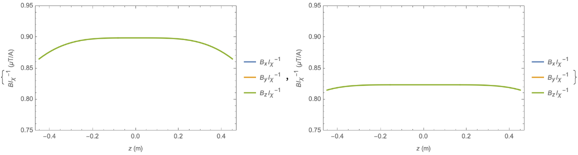 |
Optimise a saddle coil and an ellipse coil to generate the uniform transverse Bx field (encoded as the B1, 1 field harmonic):
| In[4]:= | ![{saddle, ellipse} = {First /@ InterpretationBox[FrameBox[TagBox[TooltipBox[PaneBox[GridBox[List[List[GraphicsBox[List[Thickness[0.0025`], List[FaceForm[List[RGBColor[0.9607843137254902`, 0.5058823529411764`, 0.19607843137254902`], Opacity[1.`]]], FilledCurveBox[List[List[List[0, 2, 0], List[0, 1, 0], List[0, 1, 0], List[0, 1, 0], List[0, 1, 0]], List[List[0, 2, 0], List[0, 1, 0], List[0, 1, 0], List[0, 1, 0], List[0, 1, 0]], List[List[0, 2, 0], List[0, 1, 0], List[0, 1, 0], List[0, 1, 0], List[0, 1, 0], List[0, 1, 0]], List[List[0, 2, 0], List[1, 3, 3], List[0, 1, 0], List[1, 3, 3], List[0, 1, 0], List[1, 3, 3], List[0, 1, 0], List[1, 3, 3], List[1, 3, 3], List[0, 1, 0], List[1, 3, 3], List[0, 1, 0], List[1, 3, 3]]], List[List[List[205.`, 22.863691329956055`], List[205.`, 212.31669425964355`], List[246.01799774169922`, 235.99870109558105`], List[369.0710144042969`, 307.0436840057373`], List[369.0710144042969`, 117.59068870544434`], List[205.`, 22.863691329956055`]], List[List[30.928985595703125`, 307.0436840057373`], List[153.98200225830078`, 235.99870109558105`], List[195.`, 212.31669425964355`], List[195.`, 22.863691329956055`], List[30.928985595703125`, 117.59068870544434`], List[30.928985595703125`, 307.0436840057373`]], List[List[200.`, 410.42970085144043`], List[364.0710144042969`, 315.7036876678467`], List[241.01799774169922`, 244.65868949890137`], List[200.`, 220.97669792175293`], List[158.98200225830078`, 244.65868949890137`], List[35.928985595703125`, 315.7036876678467`], List[200.`, 410.42970085144043`]], List[List[376.5710144042969`, 320.03370475769043`], List[202.5`, 420.53370475769043`], List[200.95300006866455`, 421.42667961120605`], List[199.04699993133545`, 421.42667961120605`], List[197.5`, 420.53370475769043`], List[23.428985595703125`, 320.03370475769043`], List[21.882003784179688`, 319.1406993865967`], List[20.928985595703125`, 317.4896984100342`], List[20.928985595703125`, 315.7036876678467`], List[20.928985595703125`, 114.70369529724121`], List[20.928985595703125`, 112.91769218444824`], List[21.882003784179688`, 111.26669120788574`], List[23.428985595703125`, 110.37369346618652`], List[197.5`, 9.87369155883789`], List[198.27300024032593`, 9.426692008972168`], List[199.13700008392334`, 9.203690528869629`], List[200.`, 9.203690528869629`], List[200.86299991607666`, 9.203690528869629`], List[201.72699999809265`, 9.426692008972168`], List[202.5`, 9.87369155883789`], List[376.5710144042969`, 110.37369346618652`], List[378.1179962158203`, 111.26669120788574`], List[379.0710144042969`, 112.91769218444824`], List[379.0710144042969`, 114.70369529724121`], List[379.0710144042969`, 315.7036876678467`], List[379.0710144042969`, 317.4896984100342`], List[378.1179962158203`, 319.1406993865967`], List[376.5710144042969`, 320.03370475769043`]]]]], List[FaceForm[List[RGBColor[0.5529411764705883`, 0.6745098039215687`, 0.8117647058823529`], Opacity[1.`]]], FilledCurveBox[List[List[List[0, 2, 0], List[0, 1, 0], List[0, 1, 0], List[0, 1, 0]]], List[List[List[44.92900085449219`, 282.59088134765625`], List[181.00001525878906`, 204.0298843383789`], List[181.00001525878906`, 46.90887451171875`], List[44.92900085449219`, 125.46986389160156`], List[44.92900085449219`, 282.59088134765625`]]]]], List[FaceForm[List[RGBColor[0.6627450980392157`, 0.803921568627451`, 0.5686274509803921`], Opacity[1.`]]], FilledCurveBox[List[List[List[0, 2, 0], List[0, 1, 0], List[0, 1, 0], List[0, 1, 0]]], List[List[List[355.0710144042969`, 282.59088134765625`], List[355.0710144042969`, 125.46986389160156`], List[219.`, 46.90887451171875`], List[219.`, 204.0298843383789`], List[355.0710144042969`, 282.59088134765625`]]]]], List[FaceForm[List[RGBColor[0.6901960784313725`, 0.5882352941176471`, 0.8117647058823529`], Opacity[1.`]]], FilledCurveBox[List[List[List[0, 2, 0], List[0, 1, 0], List[0, 1, 0], List[0, 1, 0]]], List[List[List[200.`, 394.0606994628906`], List[336.0710144042969`, 315.4997024536133`], List[200.`, 236.93968200683594`], List[63.928985595703125`, 315.4997024536133`], List[200.`, 394.0606994628906`]]]]]], List[Rule[BaselinePosition, Scaled[0.15`]], Rule[ImageSize, 10], Rule[ImageSize, 15]]], StyleBox[RowBox[List["FindSaddleCoil", " "]], Rule[ShowAutoStyles, False], Rule[ShowStringCharacters, False], Rule[FontSize, Times[0.9`, Inherited]], Rule[FontColor, GrayLevel[0.1`]]]]], Rule[GridBoxSpacings, List[Rule["Columns", List[List[0.25`]]]]]], Rule[Alignment, List[Left, Baseline]], Rule[BaselinePosition, Baseline], Rule[FrameMargins, List[List[3, 0], List[0, 0]]], Rule[BaseStyle, List[Rule[LineSpacing, List[0, 0]], Rule[LineBreakWithin, False]]]], RowBox[List["PacletSymbol", "[", RowBox[List["\"NoahH/CreateCoil\"", ",", "\"NoahH`CreateCoil`FindSaddleCoil\""]], "]"]], Rule[TooltipStyle, List[Rule[ShowAutoStyles, True], Rule[ShowStringCharacters, True]]]], Function[Annotation[Slot[1], Style[Defer[PacletSymbol["NoahH/CreateCoil", "NoahH`CreateCoil`FindSaddleCoil"]], Rule[ShowStringCharacters, True]], "Tooltip"]]], Rule[Background, RGBColor[0.968`, 0.976`, 0.984`]], Rule[BaselinePosition, Baseline], Rule[DefaultBaseStyle, List[]], Rule[FrameMargins, List[List[0, 0], List[1, 1]]], Rule[FrameStyle, RGBColor[0.831`, 0.847`, 0.85`]], Rule[RoundingRadius, 4]], PacletSymbol["NoahH/CreateCoil", "NoahH`CreateCoil`FindSaddleCoil"], Rule[Selectable, False], Rule[SelectWithContents, True], Rule[BoxID, "PacletSymbolBox"]][{1, -2, 2}, {1, 1}, 2, {.01, 3}], First@InterpretationBox[FrameBox[TagBox[TooltipBox[PaneBox[GridBox[List[List[GraphicsBox[List[Thickness[0.0025`], List[FaceForm[List[RGBColor[0.9607843137254902`, 0.5058823529411764`, 0.19607843137254902`], Opacity[1.`]]], FilledCurveBox[List[List[List[0, 2, 0], List[0, 1, 0], List[0, 1, 0], List[0, 1, 0], List[0, 1, 0]], List[List[0, 2, 0], List[0, 1, 0], List[0, 1, 0], List[0, 1, 0], List[0, 1, 0]], List[List[0, 2, 0], List[0, 1, 0], List[0, 1, 0], List[0, 1, 0], List[0, 1, 0], List[0, 1, 0]], List[List[0, 2, 0], List[1, 3, 3], List[0, 1, 0], List[1, 3, 3], List[0, 1, 0], List[1, 3, 3], List[0, 1, 0], List[1, 3, 3], List[1, 3, 3], List[0, 1, 0], List[1, 3, 3], List[0, 1, 0], List[1, 3, 3]]], List[List[List[205.`, 22.863691329956055`], List[205.`, 212.31669425964355`], List[246.01799774169922`, 235.99870109558105`], List[369.0710144042969`, 307.0436840057373`], List[369.0710144042969`, 117.59068870544434`], List[205.`, 22.863691329956055`]], List[List[30.928985595703125`, 307.0436840057373`], List[153.98200225830078`, 235.99870109558105`], List[195.`, 212.31669425964355`], List[195.`, 22.863691329956055`], List[30.928985595703125`, 117.59068870544434`], List[30.928985595703125`, 307.0436840057373`]], List[List[200.`, 410.42970085144043`], List[364.0710144042969`, 315.7036876678467`], List[241.01799774169922`, 244.65868949890137`], List[200.`, 220.97669792175293`], List[158.98200225830078`, 244.65868949890137`], List[35.928985595703125`, 315.7036876678467`], List[200.`, 410.42970085144043`]], List[List[376.5710144042969`, 320.03370475769043`], List[202.5`, 420.53370475769043`], List[200.95300006866455`, 421.42667961120605`], List[199.04699993133545`, 421.42667961120605`], List[197.5`, 420.53370475769043`], List[23.428985595703125`, 320.03370475769043`], List[21.882003784179688`, 319.1406993865967`], List[20.928985595703125`, 317.4896984100342`], List[20.928985595703125`, 315.7036876678467`], List[20.928985595703125`, 114.70369529724121`], List[20.928985595703125`, 112.91769218444824`], List[21.882003784179688`, 111.26669120788574`], List[23.428985595703125`, 110.37369346618652`], List[197.5`, 9.87369155883789`], List[198.27300024032593`, 9.426692008972168`], List[199.13700008392334`, 9.203690528869629`], List[200.`, 9.203690528869629`], List[200.86299991607666`, 9.203690528869629`], List[201.72699999809265`, 9.426692008972168`], List[202.5`, 9.87369155883789`], List[376.5710144042969`, 110.37369346618652`], List[378.1179962158203`, 111.26669120788574`], List[379.0710144042969`, 112.91769218444824`], List[379.0710144042969`, 114.70369529724121`], List[379.0710144042969`, 315.7036876678467`], List[379.0710144042969`, 317.4896984100342`], List[378.1179962158203`, 319.1406993865967`], List[376.5710144042969`, 320.03370475769043`]]]]], List[FaceForm[List[RGBColor[0.5529411764705883`, 0.6745098039215687`, 0.8117647058823529`], Opacity[1.`]]], FilledCurveBox[List[List[List[0, 2, 0], List[0, 1, 0], List[0, 1, 0], List[0, 1, 0]]], List[List[List[44.92900085449219`, 282.59088134765625`], List[181.00001525878906`, 204.0298843383789`], List[181.00001525878906`, 46.90887451171875`], List[44.92900085449219`, 125.46986389160156`], List[44.92900085449219`, 282.59088134765625`]]]]], List[FaceForm[List[RGBColor[0.6627450980392157`, 0.803921568627451`, 0.5686274509803921`], Opacity[1.`]]], FilledCurveBox[List[List[List[0, 2, 0], List[0, 1, 0], List[0, 1, 0], List[0, 1, 0]]], List[List[List[355.0710144042969`, 282.59088134765625`], List[355.0710144042969`, 125.46986389160156`], List[219.`, 46.90887451171875`], List[219.`, 204.0298843383789`], List[355.0710144042969`, 282.59088134765625`]]]]], List[FaceForm[List[RGBColor[0.6901960784313725`, 0.5882352941176471`, 0.8117647058823529`], Opacity[1.`]]], FilledCurveBox[List[List[List[0, 2, 0], List[0, 1, 0], List[0, 1, 0], List[0, 1, 0]]], List[List[List[200.`, 394.0606994628906`], List[336.0710144042969`, 315.4997024536133`], List[200.`, 236.93968200683594`], List[63.928985595703125`, 315.4997024536133`], List[200.`, 394.0606994628906`]]]]]], List[Rule[BaselinePosition, Scaled[0.15`]], Rule[ImageSize, 10], Rule[ImageSize, 15]]], StyleBox[RowBox[List["FindEllipseCoil", " "]], Rule[ShowAutoStyles, False], Rule[ShowStringCharacters, False], Rule[FontSize, Times[0.9`, Inherited]], Rule[FontColor, GrayLevel[0.1`]]]]], Rule[GridBoxSpacings, List[Rule["Columns", List[List[0.25`]]]]]], Rule[Alignment, List[Left, Baseline]], Rule[BaselinePosition, Baseline], Rule[FrameMargins, List[List[3, 0], List[0, 0]]], Rule[BaseStyle, List[Rule[LineSpacing, List[0, 0]], Rule[LineBreakWithin, False]]]], RowBox[List["PacletSymbol", "[", RowBox[List["\"NoahH/CreateCoil\"", ",", "\"NoahH`CreateCoil`FindEllipseCoil\""]], "]"]], Rule[TooltipStyle, List[Rule[ShowAutoStyles, True], Rule[ShowStringCharacters, True]]]], Function[Annotation[Slot[1], Style[Defer[PacletSymbol["NoahH/CreateCoil", "NoahH`CreateCoil`FindEllipseCoil"]], Rule[ShowStringCharacters, True]], "Tooltip"]]], Rule[Background, RGBColor[0.968`, 0.976`, 0.984`]], Rule[BaselinePosition, Baseline], Rule[DefaultBaseStyle, List[]], Rule[FrameMargins, List[List[0, 0], List[1, 1]]], Rule[FrameStyle, RGBColor[0.831`, 0.847`, 0.85`]], Rule[RoundingRadius, 4]], PacletSymbol["NoahH/CreateCoil", "NoahH`CreateCoil`FindEllipseCoil"], Rule[Selectable, False], Rule[SelectWithContents, True], Rule[BoxID, "PacletSymbolBox"]][{1, -1, 2}, {1, 1}, {0.1, 2}, {0.1, 0.5}]}](https://www.wolframcloud.com/obj/resourcesystem/images/a60/a60e1ebc-8364-4bbb-aa30-fb6e5a0b74a7/1-0-1/7f5323b519ccbb14.png) |
| Out[4]= |  |
Visualise the coils as 2D schematics:
| In[5]:= | ![{InterpretationBox[FrameBox[TagBox[TooltipBox[PaneBox[GridBox[List[List[GraphicsBox[List[Thickness[0.0025`], List[FaceForm[List[RGBColor[0.9607843137254902`, 0.5058823529411764`, 0.19607843137254902`], Opacity[1.`]]], FilledCurveBox[List[List[List[0, 2, 0], List[0, 1, 0], List[0, 1, 0], List[0, 1, 0], List[0, 1, 0]], List[List[0, 2, 0], List[0, 1, 0], List[0, 1, 0], List[0, 1, 0], List[0, 1, 0]], List[List[0, 2, 0], List[0, 1, 0], List[0, 1, 0], List[0, 1, 0], List[0, 1, 0], List[0, 1, 0]], List[List[0, 2, 0], List[1, 3, 3], List[0, 1, 0], List[1, 3, 3], List[0, 1, 0], List[1, 3, 3], List[0, 1, 0], List[1, 3, 3], List[1, 3, 3], List[0, 1, 0], List[1, 3, 3], List[0, 1, 0], List[1, 3, 3]]], List[List[List[205.`, 22.863691329956055`], List[205.`, 212.31669425964355`], List[246.01799774169922`, 235.99870109558105`], List[369.0710144042969`, 307.0436840057373`], List[369.0710144042969`, 117.59068870544434`], List[205.`, 22.863691329956055`]], List[List[30.928985595703125`, 307.0436840057373`], List[153.98200225830078`, 235.99870109558105`], List[195.`, 212.31669425964355`], List[195.`, 22.863691329956055`], List[30.928985595703125`, 117.59068870544434`], List[30.928985595703125`, 307.0436840057373`]], List[List[200.`, 410.42970085144043`], List[364.0710144042969`, 315.7036876678467`], List[241.01799774169922`, 244.65868949890137`], List[200.`, 220.97669792175293`], List[158.98200225830078`, 244.65868949890137`], List[35.928985595703125`, 315.7036876678467`], List[200.`, 410.42970085144043`]], List[List[376.5710144042969`, 320.03370475769043`], List[202.5`, 420.53370475769043`], List[200.95300006866455`, 421.42667961120605`], List[199.04699993133545`, 421.42667961120605`], List[197.5`, 420.53370475769043`], List[23.428985595703125`, 320.03370475769043`], List[21.882003784179688`, 319.1406993865967`], List[20.928985595703125`, 317.4896984100342`], List[20.928985595703125`, 315.7036876678467`], List[20.928985595703125`, 114.70369529724121`], List[20.928985595703125`, 112.91769218444824`], List[21.882003784179688`, 111.26669120788574`], List[23.428985595703125`, 110.37369346618652`], List[197.5`, 9.87369155883789`], List[198.27300024032593`, 9.426692008972168`], List[199.13700008392334`, 9.203690528869629`], List[200.`, 9.203690528869629`], List[200.86299991607666`, 9.203690528869629`], List[201.72699999809265`, 9.426692008972168`], List[202.5`, 9.87369155883789`], List[376.5710144042969`, 110.37369346618652`], List[378.1179962158203`, 111.26669120788574`], List[379.0710144042969`, 112.91769218444824`], List[379.0710144042969`, 114.70369529724121`], List[379.0710144042969`, 315.7036876678467`], List[379.0710144042969`, 317.4896984100342`], List[378.1179962158203`, 319.1406993865967`], List[376.5710144042969`, 320.03370475769043`]]]]], List[FaceForm[List[RGBColor[0.5529411764705883`, 0.6745098039215687`, 0.8117647058823529`], Opacity[1.`]]], FilledCurveBox[List[List[List[0, 2, 0], List[0, 1, 0], List[0, 1, 0], List[0, 1, 0]]], List[List[List[44.92900085449219`, 282.59088134765625`], List[181.00001525878906`, 204.0298843383789`], List[181.00001525878906`, 46.90887451171875`], List[44.92900085449219`, 125.46986389160156`], List[44.92900085449219`, 282.59088134765625`]]]]], List[FaceForm[List[RGBColor[0.6627450980392157`, 0.803921568627451`, 0.5686274509803921`], Opacity[1.`]]], FilledCurveBox[List[List[List[0, 2, 0], List[0, 1, 0], List[0, 1, 0], List[0, 1, 0]]], List[List[List[355.0710144042969`, 282.59088134765625`], List[355.0710144042969`, 125.46986389160156`], List[219.`, 46.90887451171875`], List[219.`, 204.0298843383789`], List[355.0710144042969`, 282.59088134765625`]]]]], List[FaceForm[List[RGBColor[0.6901960784313725`, 0.5882352941176471`, 0.8117647058823529`], Opacity[1.`]]], FilledCurveBox[List[List[List[0, 2, 0], List[0, 1, 0], List[0, 1, 0], List[0, 1, 0]]], List[List[List[200.`, 394.0606994628906`], List[336.0710144042969`, 315.4997024536133`], List[200.`, 236.93968200683594`], List[63.928985595703125`, 315.4997024536133`], List[200.`, 394.0606994628906`]]]]]], List[Rule[BaselinePosition, Scaled[0.15`]], Rule[ImageSize, 10], Rule[ImageSize, 15]]], StyleBox[RowBox[List["SaddleCoilPlot", " "]], Rule[ShowAutoStyles, False], Rule[ShowStringCharacters, False], Rule[FontSize, Times[0.9`, Inherited]], Rule[FontColor, GrayLevel[0.1`]]]]], Rule[GridBoxSpacings, List[Rule["Columns", List[List[0.25`]]]]]], Rule[Alignment, List[Left, Baseline]], Rule[BaselinePosition, Baseline], Rule[FrameMargins, List[List[3, 0], List[0, 0]]], Rule[BaseStyle, List[Rule[LineSpacing, List[0, 0]], Rule[LineBreakWithin, False]]]], RowBox[List["PacletSymbol", "[", RowBox[List["\"NoahH/CreateCoil\"", ",", "\"NoahH`CreateCoil`SaddleCoilPlot\""]], "]"]], Rule[TooltipStyle, List[Rule[ShowAutoStyles, True], Rule[ShowStringCharacters, True]]]], Function[Annotation[Slot[1], Style[Defer[PacletSymbol["NoahH/CreateCoil", "NoahH`CreateCoil`SaddleCoilPlot"]], Rule[ShowStringCharacters, True]], "Tooltip"]]], Rule[Background, RGBColor[0.968`, 0.976`, 0.984`]], Rule[BaselinePosition, Baseline], Rule[DefaultBaseStyle, List[]], Rule[FrameMargins, List[List[0, 0], List[1, 1]]], Rule[FrameStyle, RGBColor[0.831`, 0.847`, 0.85`]], Rule[RoundingRadius, 4]], PacletSymbol["NoahH/CreateCoil", "NoahH`CreateCoil`SaddleCoilPlot"], Rule[Selectable, False], Rule[SelectWithContents, True], Rule[BoxID, "PacletSymbolBox"]][saddle["AxialSeparations"], saddle["AzimuthalExtents"], {1, -2, 2}, 1, {1, 1}, ImageSize -> 450,
"ArrowheadScaling" -> .007], InterpretationBox[FrameBox[TagBox[TooltipBox[PaneBox[GridBox[List[List[GraphicsBox[List[Thickness[0.0025`], List[FaceForm[List[RGBColor[0.9607843137254902`, 0.5058823529411764`, 0.19607843137254902`], Opacity[1.`]]], FilledCurveBox[List[List[List[0, 2, 0], List[0, 1, 0], List[0, 1, 0], List[0, 1, 0], List[0, 1, 0]], List[List[0, 2, 0], List[0, 1, 0], List[0, 1, 0], List[0, 1, 0], List[0, 1, 0]], List[List[0, 2, 0], List[0, 1, 0], List[0, 1, 0], List[0, 1, 0], List[0, 1, 0], List[0, 1, 0]], List[List[0, 2, 0], List[1, 3, 3], List[0, 1, 0], List[1, 3, 3], List[0, 1, 0], List[1, 3, 3], List[0, 1, 0], List[1, 3, 3], List[1, 3, 3], List[0, 1, 0], List[1, 3, 3], List[0, 1, 0], List[1, 3, 3]]], List[List[List[205.`, 22.863691329956055`], List[205.`, 212.31669425964355`], List[246.01799774169922`, 235.99870109558105`], List[369.0710144042969`, 307.0436840057373`], List[369.0710144042969`, 117.59068870544434`], List[205.`, 22.863691329956055`]], List[List[30.928985595703125`, 307.0436840057373`], List[153.98200225830078`, 235.99870109558105`], List[195.`, 212.31669425964355`], List[195.`, 22.863691329956055`], List[30.928985595703125`, 117.59068870544434`], List[30.928985595703125`, 307.0436840057373`]], List[List[200.`, 410.42970085144043`], List[364.0710144042969`, 315.7036876678467`], List[241.01799774169922`, 244.65868949890137`], List[200.`, 220.97669792175293`], List[158.98200225830078`, 244.65868949890137`], List[35.928985595703125`, 315.7036876678467`], List[200.`, 410.42970085144043`]], List[List[376.5710144042969`, 320.03370475769043`], List[202.5`, 420.53370475769043`], List[200.95300006866455`, 421.42667961120605`], List[199.04699993133545`, 421.42667961120605`], List[197.5`, 420.53370475769043`], List[23.428985595703125`, 320.03370475769043`], List[21.882003784179688`, 319.1406993865967`], List[20.928985595703125`, 317.4896984100342`], List[20.928985595703125`, 315.7036876678467`], List[20.928985595703125`, 114.70369529724121`], List[20.928985595703125`, 112.91769218444824`], List[21.882003784179688`, 111.26669120788574`], List[23.428985595703125`, 110.37369346618652`], List[197.5`, 9.87369155883789`], List[198.27300024032593`, 9.426692008972168`], List[199.13700008392334`, 9.203690528869629`], List[200.`, 9.203690528869629`], List[200.86299991607666`, 9.203690528869629`], List[201.72699999809265`, 9.426692008972168`], List[202.5`, 9.87369155883789`], List[376.5710144042969`, 110.37369346618652`], List[378.1179962158203`, 111.26669120788574`], List[379.0710144042969`, 112.91769218444824`], List[379.0710144042969`, 114.70369529724121`], List[379.0710144042969`, 315.7036876678467`], List[379.0710144042969`, 317.4896984100342`], List[378.1179962158203`, 319.1406993865967`], List[376.5710144042969`, 320.03370475769043`]]]]], List[FaceForm[List[RGBColor[0.5529411764705883`, 0.6745098039215687`, 0.8117647058823529`], Opacity[1.`]]], FilledCurveBox[List[List[List[0, 2, 0], List[0, 1, 0], List[0, 1, 0], List[0, 1, 0]]], List[List[List[44.92900085449219`, 282.59088134765625`], List[181.00001525878906`, 204.0298843383789`], List[181.00001525878906`, 46.90887451171875`], List[44.92900085449219`, 125.46986389160156`], List[44.92900085449219`, 282.59088134765625`]]]]], List[FaceForm[List[RGBColor[0.6627450980392157`, 0.803921568627451`, 0.5686274509803921`], Opacity[1.`]]], FilledCurveBox[List[List[List[0, 2, 0], List[0, 1, 0], List[0, 1, 0], List[0, 1, 0]]], List[List[List[355.0710144042969`, 282.59088134765625`], List[355.0710144042969`, 125.46986389160156`], List[219.`, 46.90887451171875`], List[219.`, 204.0298843383789`], List[355.0710144042969`, 282.59088134765625`]]]]], List[FaceForm[List[RGBColor[0.6901960784313725`, 0.5882352941176471`, 0.8117647058823529`], Opacity[1.`]]], FilledCurveBox[List[List[List[0, 2, 0], List[0, 1, 0], List[0, 1, 0], List[0, 1, 0]]], List[List[List[200.`, 394.0606994628906`], List[336.0710144042969`, 315.4997024536133`], List[200.`, 236.93968200683594`], List[63.928985595703125`, 315.4997024536133`], List[200.`, 394.0606994628906`]]]]]], List[Rule[BaselinePosition, Scaled[0.15`]], Rule[ImageSize, 10], Rule[ImageSize, 15]]], StyleBox[RowBox[List["EllipseCoilPlot", " "]], Rule[ShowAutoStyles, False], Rule[ShowStringCharacters, False], Rule[FontSize, Times[0.9`, Inherited]], Rule[FontColor, GrayLevel[0.1`]]]]], Rule[GridBoxSpacings, List[Rule["Columns", List[List[0.25`]]]]]], Rule[Alignment, List[Left, Baseline]], Rule[BaselinePosition, Baseline], Rule[FrameMargins, List[List[3, 0], List[0, 0]]], Rule[BaseStyle, List[Rule[LineSpacing, List[0, 0]], Rule[LineBreakWithin, False]]]], RowBox[List["PacletSymbol", "[", RowBox[List["\"NoahH/CreateCoil\"", ",", "\"NoahH`CreateCoil`EllipseCoilPlot\""]], "]"]], Rule[TooltipStyle, List[Rule[ShowAutoStyles, True], Rule[ShowStringCharacters, True]]]], Function[Annotation[Slot[1], Style[Defer[PacletSymbol["NoahH/CreateCoil", "NoahH`CreateCoil`EllipseCoilPlot"]], Rule[ShowStringCharacters, True]], "Tooltip"]]], Rule[Background, RGBColor[0.968`, 0.976`, 0.984`]], Rule[BaselinePosition, Baseline], Rule[DefaultBaseStyle, List[]], Rule[FrameMargins, List[List[0, 0], List[1, 1]]], Rule[FrameStyle, RGBColor[0.831`, 0.847`, 0.85`]], Rule[RoundingRadius, 4]], PacletSymbol["NoahH/CreateCoil", "NoahH`CreateCoil`EllipseCoilPlot"], Rule[Selectable, False], Rule[SelectWithContents, True], Rule[BoxID, "PacletSymbolBox"]][ellipse, {1, -1, 2}, 1, {1, 1}, ImageSize -> 450, "ArrowheadScaling" -> .007]}](https://www.wolframcloud.com/obj/resourcesystem/images/a60/a60e1ebc-8364-4bbb-aa30-fb6e5a0b74a7/1-0-1/17d1167ba874351c.png) |
| Out[5]= | 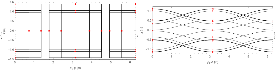 |
Visualise the coils as 3D plots. Colour each ellipse primitive differently to distinguish them more easily:
| In[6]:= | ![{InterpretationBox[FrameBox[TagBox[TooltipBox[PaneBox[GridBox[List[List[GraphicsBox[List[Thickness[0.0025`], List[FaceForm[List[RGBColor[0.9607843137254902`, 0.5058823529411764`, 0.19607843137254902`], Opacity[1.`]]], FilledCurveBox[List[List[List[0, 2, 0], List[0, 1, 0], List[0, 1, 0], List[0, 1, 0], List[0, 1, 0]], List[List[0, 2, 0], List[0, 1, 0], List[0, 1, 0], List[0, 1, 0], List[0, 1, 0]], List[List[0, 2, 0], List[0, 1, 0], List[0, 1, 0], List[0, 1, 0], List[0, 1, 0], List[0, 1, 0]], List[List[0, 2, 0], List[1, 3, 3], List[0, 1, 0], List[1, 3, 3], List[0, 1, 0], List[1, 3, 3], List[0, 1, 0], List[1, 3, 3], List[1, 3, 3], List[0, 1, 0], List[1, 3, 3], List[0, 1, 0], List[1, 3, 3]]], List[List[List[205.`, 22.863691329956055`], List[205.`, 212.31669425964355`], List[246.01799774169922`, 235.99870109558105`], List[369.0710144042969`, 307.0436840057373`], List[369.0710144042969`, 117.59068870544434`], List[205.`, 22.863691329956055`]], List[List[30.928985595703125`, 307.0436840057373`], List[153.98200225830078`, 235.99870109558105`], List[195.`, 212.31669425964355`], List[195.`, 22.863691329956055`], List[30.928985595703125`, 117.59068870544434`], List[30.928985595703125`, 307.0436840057373`]], List[List[200.`, 410.42970085144043`], List[364.0710144042969`, 315.7036876678467`], List[241.01799774169922`, 244.65868949890137`], List[200.`, 220.97669792175293`], List[158.98200225830078`, 244.65868949890137`], List[35.928985595703125`, 315.7036876678467`], List[200.`, 410.42970085144043`]], List[List[376.5710144042969`, 320.03370475769043`], List[202.5`, 420.53370475769043`], List[200.95300006866455`, 421.42667961120605`], List[199.04699993133545`, 421.42667961120605`], List[197.5`, 420.53370475769043`], List[23.428985595703125`, 320.03370475769043`], List[21.882003784179688`, 319.1406993865967`], List[20.928985595703125`, 317.4896984100342`], List[20.928985595703125`, 315.7036876678467`], List[20.928985595703125`, 114.70369529724121`], List[20.928985595703125`, 112.91769218444824`], List[21.882003784179688`, 111.26669120788574`], List[23.428985595703125`, 110.37369346618652`], List[197.5`, 9.87369155883789`], List[198.27300024032593`, 9.426692008972168`], List[199.13700008392334`, 9.203690528869629`], List[200.`, 9.203690528869629`], List[200.86299991607666`, 9.203690528869629`], List[201.72699999809265`, 9.426692008972168`], List[202.5`, 9.87369155883789`], List[376.5710144042969`, 110.37369346618652`], List[378.1179962158203`, 111.26669120788574`], List[379.0710144042969`, 112.91769218444824`], List[379.0710144042969`, 114.70369529724121`], List[379.0710144042969`, 315.7036876678467`], List[379.0710144042969`, 317.4896984100342`], List[378.1179962158203`, 319.1406993865967`], List[376.5710144042969`, 320.03370475769043`]]]]], List[FaceForm[List[RGBColor[0.5529411764705883`, 0.6745098039215687`, 0.8117647058823529`], Opacity[1.`]]], FilledCurveBox[List[List[List[0, 2, 0], List[0, 1, 0], List[0, 1, 0], List[0, 1, 0]]], List[List[List[44.92900085449219`, 282.59088134765625`], List[181.00001525878906`, 204.0298843383789`], List[181.00001525878906`, 46.90887451171875`], List[44.92900085449219`, 125.46986389160156`], List[44.92900085449219`, 282.59088134765625`]]]]], List[FaceForm[List[RGBColor[0.6627450980392157`, 0.803921568627451`, 0.5686274509803921`], Opacity[1.`]]], FilledCurveBox[List[List[List[0, 2, 0], List[0, 1, 0], List[0, 1, 0], List[0, 1, 0]]], List[List[List[355.0710144042969`, 282.59088134765625`], List[355.0710144042969`, 125.46986389160156`], List[219.`, 46.90887451171875`], List[219.`, 204.0298843383789`], List[355.0710144042969`, 282.59088134765625`]]]]], List[FaceForm[List[RGBColor[0.6901960784313725`, 0.5882352941176471`, 0.8117647058823529`], Opacity[1.`]]], FilledCurveBox[List[List[List[0, 2, 0], List[0, 1, 0], List[0, 1, 0], List[0, 1, 0]]], List[List[List[200.`, 394.0606994628906`], List[336.0710144042969`, 315.4997024536133`], List[200.`, 236.93968200683594`], List[63.928985595703125`, 315.4997024536133`], List[200.`, 394.0606994628906`]]]]]], List[Rule[BaselinePosition, Scaled[0.15`]], Rule[ImageSize, 10], Rule[ImageSize, 15]]], StyleBox[RowBox[List["SaddleCoilPlot3D", " "]], Rule[ShowAutoStyles, False], Rule[ShowStringCharacters, False], Rule[FontSize, Times[0.9`, Inherited]], Rule[FontColor, GrayLevel[0.1`]]]]], Rule[GridBoxSpacings, List[Rule["Columns", List[List[0.25`]]]]]], Rule[Alignment, List[Left, Baseline]], Rule[BaselinePosition, Baseline], Rule[FrameMargins, List[List[3, 0], List[0, 0]]], Rule[BaseStyle, List[Rule[LineSpacing, List[0, 0]], Rule[LineBreakWithin, False]]]], RowBox[List["PacletSymbol", "[", RowBox[List["\"NoahH/CreateCoil\"", ",", "\"NoahH`CreateCoil`SaddleCoilPlot3D\""]], "]"]], Rule[TooltipStyle, List[Rule[ShowAutoStyles, True], Rule[ShowStringCharacters, True]]]], Function[Annotation[Slot[1], Style[Defer[PacletSymbol["NoahH/CreateCoil", "NoahH`CreateCoil`SaddleCoilPlot3D"]], Rule[ShowStringCharacters, True]], "Tooltip"]]], Rule[Background, RGBColor[0.968`, 0.976`, 0.984`]], Rule[BaselinePosition, Baseline], Rule[DefaultBaseStyle, List[]], Rule[FrameMargins, List[List[0, 0], List[1, 1]]], Rule[FrameStyle, RGBColor[0.831`, 0.847`, 0.85`]], Rule[RoundingRadius, 4]], PacletSymbol["NoahH/CreateCoil", "NoahH`CreateCoil`SaddleCoilPlot3D"], Rule[Selectable, False], Rule[SelectWithContents, True], Rule[BoxID, "PacletSymbolBox"]][saddle["AxialSeparations"], saddle["AzimuthalExtents"], {1, -2, 2}, 1, {1, 1}, ImageSize -> 450,
"ThicknessScaling" -> .002],
InterpretationBox[FrameBox[TagBox[TooltipBox[PaneBox[GridBox[List[List[GraphicsBox[List[Thickness[0.0025`], List[FaceForm[List[RGBColor[0.9607843137254902`, 0.5058823529411764`, 0.19607843137254902`], Opacity[1.`]]], FilledCurveBox[List[List[List[0, 2, 0], List[0, 1, 0], List[0, 1, 0], List[0, 1, 0], List[0, 1, 0]], List[List[0, 2, 0], List[0, 1, 0], List[0, 1, 0], List[0, 1, 0], List[0, 1, 0]], List[List[0, 2, 0], List[0, 1, 0], List[0, 1, 0], List[0, 1, 0], List[0, 1, 0], List[0, 1, 0]], List[List[0, 2, 0], List[1, 3, 3], List[0, 1, 0], List[1, 3, 3], List[0, 1, 0], List[1, 3, 3], List[0, 1, 0], List[1, 3, 3], List[1, 3, 3], List[0, 1, 0], List[1, 3, 3], List[0, 1, 0], List[1, 3, 3]]], List[List[List[205.`, 22.863691329956055`], List[205.`, 212.31669425964355`], List[246.01799774169922`, 235.99870109558105`], List[369.0710144042969`, 307.0436840057373`], List[369.0710144042969`, 117.59068870544434`], List[205.`, 22.863691329956055`]], List[List[30.928985595703125`, 307.0436840057373`], List[153.98200225830078`, 235.99870109558105`], List[195.`, 212.31669425964355`], List[195.`, 22.863691329956055`], List[30.928985595703125`, 117.59068870544434`], List[30.928985595703125`, 307.0436840057373`]], List[List[200.`, 410.42970085144043`], List[364.0710144042969`, 315.7036876678467`], List[241.01799774169922`, 244.65868949890137`], List[200.`, 220.97669792175293`], List[158.98200225830078`, 244.65868949890137`], List[35.928985595703125`, 315.7036876678467`], List[200.`, 410.42970085144043`]], List[List[376.5710144042969`, 320.03370475769043`], List[202.5`, 420.53370475769043`], List[200.95300006866455`, 421.42667961120605`], List[199.04699993133545`, 421.42667961120605`], List[197.5`, 420.53370475769043`], List[23.428985595703125`, 320.03370475769043`], List[21.882003784179688`, 319.1406993865967`], List[20.928985595703125`, 317.4896984100342`], List[20.928985595703125`, 315.7036876678467`], List[20.928985595703125`, 114.70369529724121`], List[20.928985595703125`, 112.91769218444824`], List[21.882003784179688`, 111.26669120788574`], List[23.428985595703125`, 110.37369346618652`], List[197.5`, 9.87369155883789`], List[198.27300024032593`, 9.426692008972168`], List[199.13700008392334`, 9.203690528869629`], List[200.`, 9.203690528869629`], List[200.86299991607666`, 9.203690528869629`], List[201.72699999809265`, 9.426692008972168`], List[202.5`, 9.87369155883789`], List[376.5710144042969`, 110.37369346618652`], List[378.1179962158203`, 111.26669120788574`], List[379.0710144042969`, 112.91769218444824`], List[379.0710144042969`, 114.70369529724121`], List[379.0710144042969`, 315.7036876678467`], List[379.0710144042969`, 317.4896984100342`], List[378.1179962158203`, 319.1406993865967`], List[376.5710144042969`, 320.03370475769043`]]]]], List[FaceForm[List[RGBColor[0.5529411764705883`, 0.6745098039215687`, 0.8117647058823529`], Opacity[1.`]]], FilledCurveBox[List[List[List[0, 2, 0], List[0, 1, 0], List[0, 1, 0], List[0, 1, 0]]], List[List[List[44.92900085449219`, 282.59088134765625`], List[181.00001525878906`, 204.0298843383789`], List[181.00001525878906`, 46.90887451171875`], List[44.92900085449219`, 125.46986389160156`], List[44.92900085449219`, 282.59088134765625`]]]]], List[FaceForm[List[RGBColor[0.6627450980392157`, 0.803921568627451`, 0.5686274509803921`], Opacity[1.`]]], FilledCurveBox[List[List[List[0, 2, 0], List[0, 1, 0], List[0, 1, 0], List[0, 1, 0]]], List[List[List[355.0710144042969`, 282.59088134765625`], List[355.0710144042969`, 125.46986389160156`], List[219.`, 46.90887451171875`], List[219.`, 204.0298843383789`], List[355.0710144042969`, 282.59088134765625`]]]]], List[FaceForm[List[RGBColor[0.6901960784313725`, 0.5882352941176471`, 0.8117647058823529`], Opacity[1.`]]], FilledCurveBox[List[List[List[0, 2, 0], List[0, 1, 0], List[0, 1, 0], List[0, 1, 0]]], List[List[List[200.`, 394.0606994628906`], List[336.0710144042969`, 315.4997024536133`], List[200.`, 236.93968200683594`], List[63.928985595703125`, 315.4997024536133`], List[200.`, 394.0606994628906`]]]]]], List[Rule[BaselinePosition, Scaled[0.15`]], Rule[ImageSize, 10], Rule[ImageSize, 15]]], StyleBox[RowBox[List["EllipseCoilPlot3D", " "]], Rule[ShowAutoStyles, False], Rule[ShowStringCharacters, False], Rule[FontSize, Times[0.9`, Inherited]], Rule[FontColor, GrayLevel[0.1`]]]]], Rule[GridBoxSpacings, List[Rule["Columns", List[List[0.25`]]]]]], Rule[Alignment, List[Left, Baseline]], Rule[BaselinePosition, Baseline], Rule[FrameMargins, List[List[3, 0], List[0, 0]]], Rule[BaseStyle, List[Rule[LineSpacing, List[0, 0]], Rule[LineBreakWithin, False]]]], RowBox[List["PacletSymbol", "[", RowBox[List["\"NoahH/CreateCoil\"", ",", "\"NoahH`CreateCoil`EllipseCoilPlot3D\""]], "]"]], Rule[TooltipStyle, List[Rule[ShowAutoStyles, True], Rule[ShowStringCharacters, True]]]], Function[Annotation[Slot[1], Style[Defer[PacletSymbol["NoahH/CreateCoil", "NoahH`CreateCoil`EllipseCoilPlot3D"]], Rule[ShowStringCharacters, True]], "Tooltip"]]], Rule[Background, RGBColor[0.968`, 0.976`, 0.984`]], Rule[BaselinePosition, Baseline], Rule[DefaultBaseStyle, List[]], Rule[FrameMargins, List[List[0, 0], List[1, 1]]], Rule[FrameStyle, RGBColor[0.831`, 0.847`, 0.85`]], Rule[RoundingRadius, 4]], PacletSymbol["NoahH/CreateCoil", "NoahH`CreateCoil`EllipseCoilPlot3D"], Rule[Selectable, False], Rule[SelectWithContents, True], Rule[BoxID, "PacletSymbolBox"]][ellipse, {1, -1, 2}, 1, {1, 1}, ImageSize -> 450, "ThicknessScaling" -> .0035, PlotStyle -> Automatic]}](https://www.wolframcloud.com/obj/resourcesystem/images/a60/a60e1ebc-8364-4bbb-aa30-fb6e5a0b74a7/1-0-1/10599e96aa10356b.png) |
| Out[6]= | 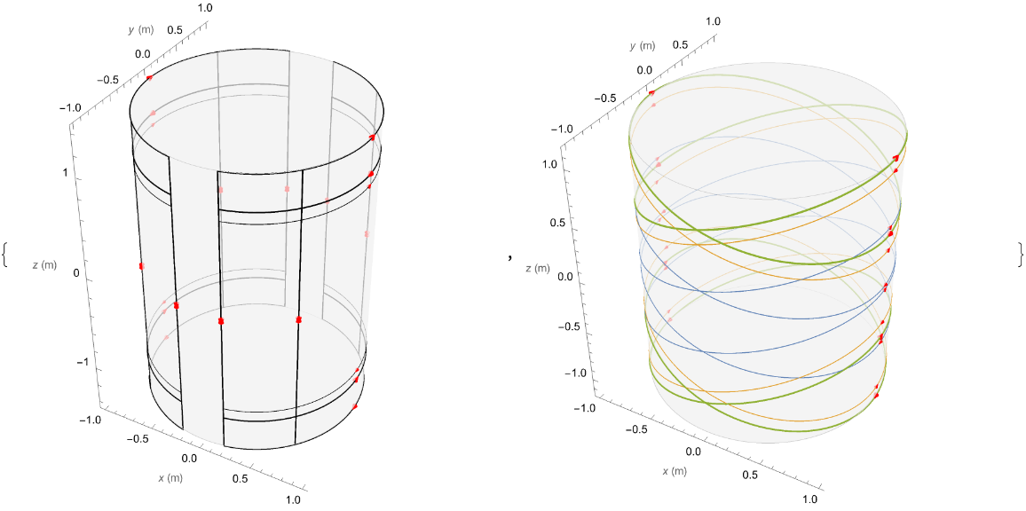 |
Plot the Bx field component generated by each coil in the xz-plane:
| In[7]:= | ![{InterpretationBox[FrameBox[TagBox[TooltipBox[PaneBox[GridBox[List[List[GraphicsBox[List[Thickness[0.0025`], List[FaceForm[List[RGBColor[0.9607843137254902`, 0.5058823529411764`, 0.19607843137254902`], Opacity[1.`]]], FilledCurveBox[List[List[List[0, 2, 0], List[0, 1, 0], List[0, 1, 0], List[0, 1, 0], List[0, 1, 0]], List[List[0, 2, 0], List[0, 1, 0], List[0, 1, 0], List[0, 1, 0], List[0, 1, 0]], List[List[0, 2, 0], List[0, 1, 0], List[0, 1, 0], List[0, 1, 0], List[0, 1, 0], List[0, 1, 0]], List[List[0, 2, 0], List[1, 3, 3], List[0, 1, 0], List[1, 3, 3], List[0, 1, 0], List[1, 3, 3], List[0, 1, 0], List[1, 3, 3], List[1, 3, 3], List[0, 1, 0], List[1, 3, 3], List[0, 1, 0], List[1, 3, 3]]], List[List[List[205.`, 22.863691329956055`], List[205.`, 212.31669425964355`], List[246.01799774169922`, 235.99870109558105`], List[369.0710144042969`, 307.0436840057373`], List[369.0710144042969`, 117.59068870544434`], List[205.`, 22.863691329956055`]], List[List[30.928985595703125`, 307.0436840057373`], List[153.98200225830078`, 235.99870109558105`], List[195.`, 212.31669425964355`], List[195.`, 22.863691329956055`], List[30.928985595703125`, 117.59068870544434`], List[30.928985595703125`, 307.0436840057373`]], List[List[200.`, 410.42970085144043`], List[364.0710144042969`, 315.7036876678467`], List[241.01799774169922`, 244.65868949890137`], List[200.`, 220.97669792175293`], List[158.98200225830078`, 244.65868949890137`], List[35.928985595703125`, 315.7036876678467`], List[200.`, 410.42970085144043`]], List[List[376.5710144042969`, 320.03370475769043`], List[202.5`, 420.53370475769043`], List[200.95300006866455`, 421.42667961120605`], List[199.04699993133545`, 421.42667961120605`], List[197.5`, 420.53370475769043`], List[23.428985595703125`, 320.03370475769043`], List[21.882003784179688`, 319.1406993865967`], List[20.928985595703125`, 317.4896984100342`], List[20.928985595703125`, 315.7036876678467`], List[20.928985595703125`, 114.70369529724121`], List[20.928985595703125`, 112.91769218444824`], List[21.882003784179688`, 111.26669120788574`], List[23.428985595703125`, 110.37369346618652`], List[197.5`, 9.87369155883789`], List[198.27300024032593`, 9.426692008972168`], List[199.13700008392334`, 9.203690528869629`], List[200.`, 9.203690528869629`], List[200.86299991607666`, 9.203690528869629`], List[201.72699999809265`, 9.426692008972168`], List[202.5`, 9.87369155883789`], List[376.5710144042969`, 110.37369346618652`], List[378.1179962158203`, 111.26669120788574`], List[379.0710144042969`, 112.91769218444824`], List[379.0710144042969`, 114.70369529724121`], List[379.0710144042969`, 315.7036876678467`], List[379.0710144042969`, 317.4896984100342`], List[378.1179962158203`, 319.1406993865967`], List[376.5710144042969`, 320.03370475769043`]]]]], List[FaceForm[List[RGBColor[0.5529411764705883`, 0.6745098039215687`, 0.8117647058823529`], Opacity[1.`]]], FilledCurveBox[List[List[List[0, 2, 0], List[0, 1, 0], List[0, 1, 0], List[0, 1, 0]]], List[List[List[44.92900085449219`, 282.59088134765625`], List[181.00001525878906`, 204.0298843383789`], List[181.00001525878906`, 46.90887451171875`], List[44.92900085449219`, 125.46986389160156`], List[44.92900085449219`, 282.59088134765625`]]]]], List[FaceForm[List[RGBColor[0.6627450980392157`, 0.803921568627451`, 0.5686274509803921`], Opacity[1.`]]], FilledCurveBox[List[List[List[0, 2, 0], List[0, 1, 0], List[0, 1, 0], List[0, 1, 0]]], List[List[List[355.0710144042969`, 282.59088134765625`], List[355.0710144042969`, 125.46986389160156`], List[219.`, 46.90887451171875`], List[219.`, 204.0298843383789`], List[355.0710144042969`, 282.59088134765625`]]]]], List[FaceForm[List[RGBColor[0.6901960784313725`, 0.5882352941176471`, 0.8117647058823529`], Opacity[1.`]]], FilledCurveBox[List[List[List[0, 2, 0], List[0, 1, 0], List[0, 1, 0], List[0, 1, 0]]], List[List[List[200.`, 394.0606994628906`], List[336.0710144042969`, 315.4997024536133`], List[200.`, 236.93968200683594`], List[63.928985595703125`, 315.4997024536133`], List[200.`, 394.0606994628906`]]]]]], List[Rule[BaselinePosition, Scaled[0.15`]], Rule[ImageSize, 10], Rule[ImageSize, 15]]], StyleBox[RowBox[List["SaddleFieldPlot2D", " "]], Rule[ShowAutoStyles, False], Rule[ShowStringCharacters, False], Rule[FontSize, Times[0.9`, Inherited]], Rule[FontColor, GrayLevel[0.1`]]]]], Rule[GridBoxSpacings, List[Rule["Columns", List[List[0.25`]]]]]], Rule[Alignment, List[Left, Baseline]], Rule[BaselinePosition, Baseline], Rule[FrameMargins, List[List[3, 0], List[0, 0]]], Rule[BaseStyle, List[Rule[LineSpacing, List[0, 0]], Rule[LineBreakWithin, False]]]], RowBox[List["PacletSymbol", "[", RowBox[List["\"NoahH/CreateCoil\"", ",", "\"NoahH`CreateCoil`SaddleFieldPlot2D\""]], "]"]], Rule[TooltipStyle, List[Rule[ShowAutoStyles, True], Rule[ShowStringCharacters, True]]]], Function[Annotation[Slot[1], Style[Defer[PacletSymbol["NoahH/CreateCoil", "NoahH`CreateCoil`SaddleFieldPlot2D"]], Rule[ShowStringCharacters, True]], "Tooltip"]]], Rule[Background, RGBColor[0.968`, 0.976`, 0.984`]], Rule[BaselinePosition, Baseline], Rule[DefaultBaseStyle, List[]], Rule[FrameMargins, List[List[0, 0], List[1, 1]]], Rule[FrameStyle, RGBColor[0.831`, 0.847`, 0.85`]], Rule[RoundingRadius, 4]], PacletSymbol["NoahH/CreateCoil", "NoahH`CreateCoil`SaddleFieldPlot2D"], Rule[Selectable, False], Rule[SelectWithContents, True], Rule[BoxID, "PacletSymbolBox"]][saddle["AxialSeparations"], saddle["AzimuthalExtents"], {1, -2, 2}, 1, {1, 1}, ImageSize -> 370][[1]],
InterpretationBox[FrameBox[TagBox[TooltipBox[PaneBox[GridBox[List[List[GraphicsBox[List[Thickness[0.0025`], List[FaceForm[List[RGBColor[0.9607843137254902`, 0.5058823529411764`, 0.19607843137254902`], Opacity[1.`]]], FilledCurveBox[List[List[List[0, 2, 0], List[0, 1, 0], List[0, 1, 0], List[0, 1, 0], List[0, 1, 0]], List[List[0, 2, 0], List[0, 1, 0], List[0, 1, 0], List[0, 1, 0], List[0, 1, 0]], List[List[0, 2, 0], List[0, 1, 0], List[0, 1, 0], List[0, 1, 0], List[0, 1, 0], List[0, 1, 0]], List[List[0, 2, 0], List[1, 3, 3], List[0, 1, 0], List[1, 3, 3], List[0, 1, 0], List[1, 3, 3], List[0, 1, 0], List[1, 3, 3], List[1, 3, 3], List[0, 1, 0], List[1, 3, 3], List[0, 1, 0], List[1, 3, 3]]], List[List[List[205.`, 22.863691329956055`], List[205.`, 212.31669425964355`], List[246.01799774169922`, 235.99870109558105`], List[369.0710144042969`, 307.0436840057373`], List[369.0710144042969`, 117.59068870544434`], List[205.`, 22.863691329956055`]], List[List[30.928985595703125`, 307.0436840057373`], List[153.98200225830078`, 235.99870109558105`], List[195.`, 212.31669425964355`], List[195.`, 22.863691329956055`], List[30.928985595703125`, 117.59068870544434`], List[30.928985595703125`, 307.0436840057373`]], List[List[200.`, 410.42970085144043`], List[364.0710144042969`, 315.7036876678467`], List[241.01799774169922`, 244.65868949890137`], List[200.`, 220.97669792175293`], List[158.98200225830078`, 244.65868949890137`], List[35.928985595703125`, 315.7036876678467`], List[200.`, 410.42970085144043`]], List[List[376.5710144042969`, 320.03370475769043`], List[202.5`, 420.53370475769043`], List[200.95300006866455`, 421.42667961120605`], List[199.04699993133545`, 421.42667961120605`], List[197.5`, 420.53370475769043`], List[23.428985595703125`, 320.03370475769043`], List[21.882003784179688`, 319.1406993865967`], List[20.928985595703125`, 317.4896984100342`], List[20.928985595703125`, 315.7036876678467`], List[20.928985595703125`, 114.70369529724121`], List[20.928985595703125`, 112.91769218444824`], List[21.882003784179688`, 111.26669120788574`], List[23.428985595703125`, 110.37369346618652`], List[197.5`, 9.87369155883789`], List[198.27300024032593`, 9.426692008972168`], List[199.13700008392334`, 9.203690528869629`], List[200.`, 9.203690528869629`], List[200.86299991607666`, 9.203690528869629`], List[201.72699999809265`, 9.426692008972168`], List[202.5`, 9.87369155883789`], List[376.5710144042969`, 110.37369346618652`], List[378.1179962158203`, 111.26669120788574`], List[379.0710144042969`, 112.91769218444824`], List[379.0710144042969`, 114.70369529724121`], List[379.0710144042969`, 315.7036876678467`], List[379.0710144042969`, 317.4896984100342`], List[378.1179962158203`, 319.1406993865967`], List[376.5710144042969`, 320.03370475769043`]]]]], List[FaceForm[List[RGBColor[0.5529411764705883`, 0.6745098039215687`, 0.8117647058823529`], Opacity[1.`]]], FilledCurveBox[List[List[List[0, 2, 0], List[0, 1, 0], List[0, 1, 0], List[0, 1, 0]]], List[List[List[44.92900085449219`, 282.59088134765625`], List[181.00001525878906`, 204.0298843383789`], List[181.00001525878906`, 46.90887451171875`], List[44.92900085449219`, 125.46986389160156`], List[44.92900085449219`, 282.59088134765625`]]]]], List[FaceForm[List[RGBColor[0.6627450980392157`, 0.803921568627451`, 0.5686274509803921`], Opacity[1.`]]], FilledCurveBox[List[List[List[0, 2, 0], List[0, 1, 0], List[0, 1, 0], List[0, 1, 0]]], List[List[List[355.0710144042969`, 282.59088134765625`], List[355.0710144042969`, 125.46986389160156`], List[219.`, 46.90887451171875`], List[219.`, 204.0298843383789`], List[355.0710144042969`, 282.59088134765625`]]]]], List[FaceForm[List[RGBColor[0.6901960784313725`, 0.5882352941176471`, 0.8117647058823529`], Opacity[1.`]]], FilledCurveBox[List[List[List[0, 2, 0], List[0, 1, 0], List[0, 1, 0], List[0, 1, 0]]], List[List[List[200.`, 394.0606994628906`], List[336.0710144042969`, 315.4997024536133`], List[200.`, 236.93968200683594`], List[63.928985595703125`, 315.4997024536133`], List[200.`, 394.0606994628906`]]]]]], List[Rule[BaselinePosition, Scaled[0.15`]], Rule[ImageSize, 10], Rule[ImageSize, 15]]], StyleBox[RowBox[List["EllipseFieldPlot2D", " "]], Rule[ShowAutoStyles, False], Rule[ShowStringCharacters, False], Rule[FontSize, Times[0.9`, Inherited]], Rule[FontColor, GrayLevel[0.1`]]]]], Rule[GridBoxSpacings, List[Rule["Columns", List[List[0.25`]]]]]], Rule[Alignment, List[Left, Baseline]], Rule[BaselinePosition, Baseline], Rule[FrameMargins, List[List[3, 0], List[0, 0]]], Rule[BaseStyle, List[Rule[LineSpacing, List[0, 0]], Rule[LineBreakWithin, False]]]], RowBox[List["PacletSymbol", "[", RowBox[List["\"NoahH/CreateCoil\"", ",", "\"NoahH`CreateCoil`EllipseFieldPlot2D\""]], "]"]], Rule[TooltipStyle, List[Rule[ShowAutoStyles, True], Rule[ShowStringCharacters, True]]]], Function[Annotation[Slot[1], Style[Defer[PacletSymbol["NoahH/CreateCoil", "NoahH`CreateCoil`EllipseFieldPlot2D"]], Rule[ShowStringCharacters, True]], "Tooltip"]]], Rule[Background, RGBColor[0.968`, 0.976`, 0.984`]], Rule[BaselinePosition, Baseline], Rule[DefaultBaseStyle, List[]], Rule[FrameMargins, List[List[0, 0], List[1, 1]]], Rule[FrameStyle, RGBColor[0.831`, 0.847`, 0.85`]], Rule[RoundingRadius, 4]], PacletSymbol["NoahH/CreateCoil", "NoahH`CreateCoil`EllipseFieldPlot2D"], Rule[Selectable, False], Rule[SelectWithContents, True], Rule[BoxID, "PacletSymbolBox"]][ellipse, {1, -1, 2}, 1, {1, 1}, ImageSize -> 370][[1]]}](https://www.wolframcloud.com/obj/resourcesystem/images/a60/a60e1ebc-8364-4bbb-aa30-fb6e5a0b74a7/1-0-1/5d27e21cdf400c17.png) |
| Out[8]= | 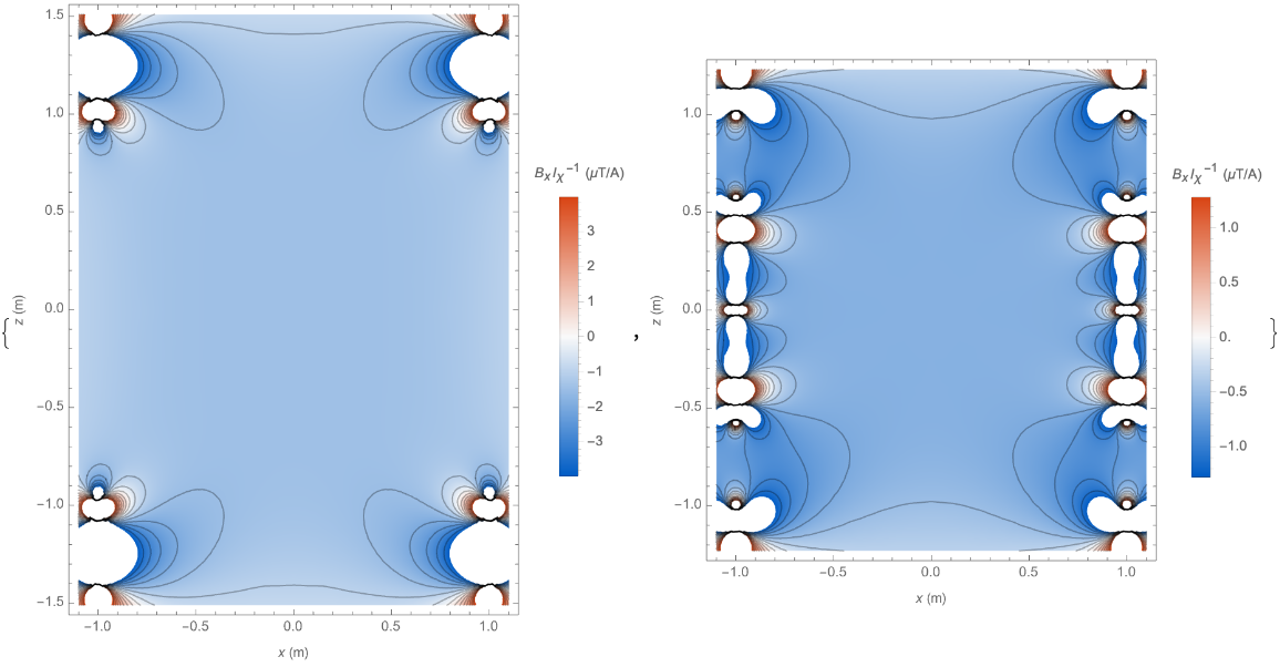 |
The search domain can be constrained to account for physical constraints. Optimise a loop coil of three pairs to generate the B2, 0 field harmonic, with axial separations constrained between 0.5 and 1 times the coil radius:
| In[9]:= |
| Out[9]= |  |
| In[10]:= |
| Out[10]= | 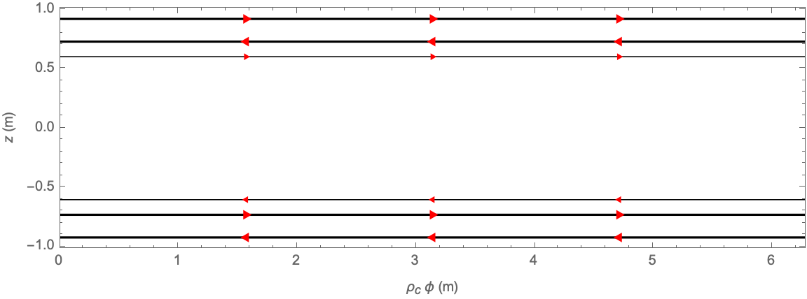 |
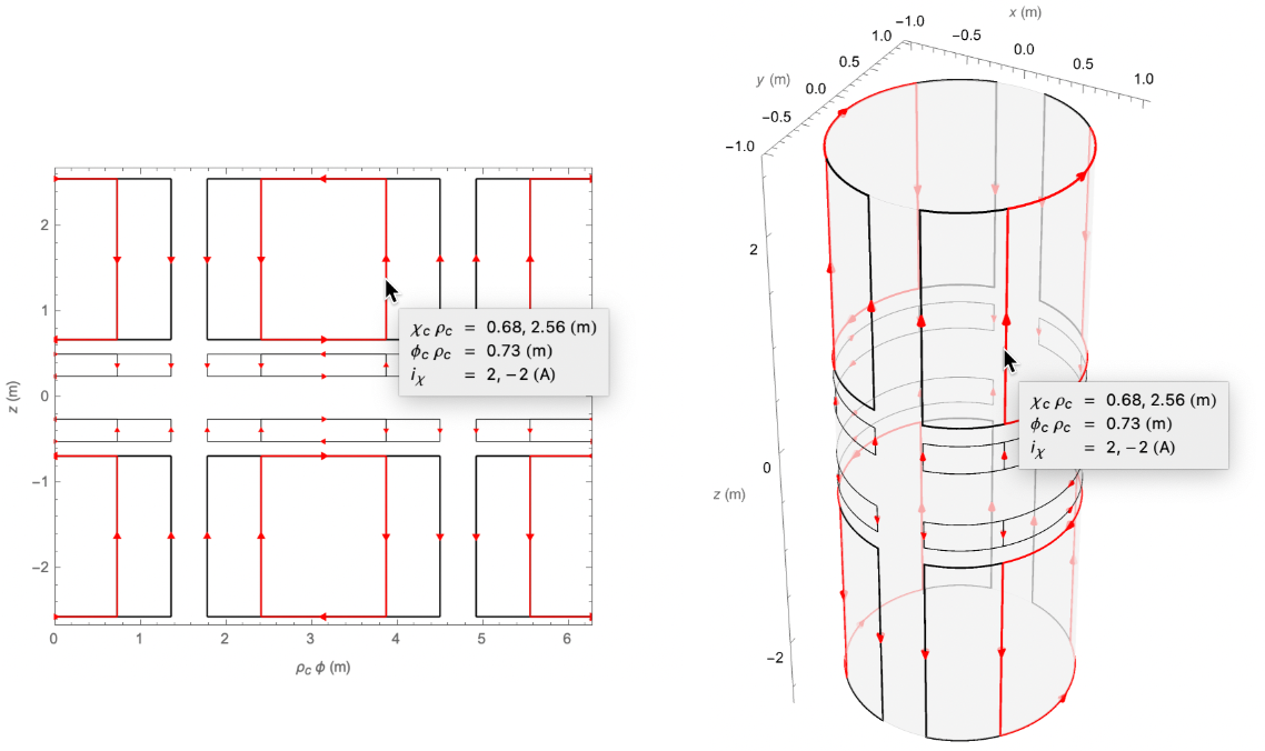
When the mouse hovers over a wire in a 2D or 3D coil plot, all other wires belonging to the same coil primitive are highlighted, and a tooltip shows the parameters describing that primitive:
By default, FindLoopCoil, FindSaddleCoil, and FindEllipseCoil null one fewer leading-order error field harmonics than there are coil parameters, meaning that solutions lie on a 1D contour embedded in a solution space whose dimensionality is equal to the number of coil parameters. Points are found on the solution contour by searching over a coarse mesh of search seeds. These points are interpolated to produce a fine mesh of search seeds, which yield the final set of solutions:
| In[11]:= |
| In[12]:= |
| Out[12]= | 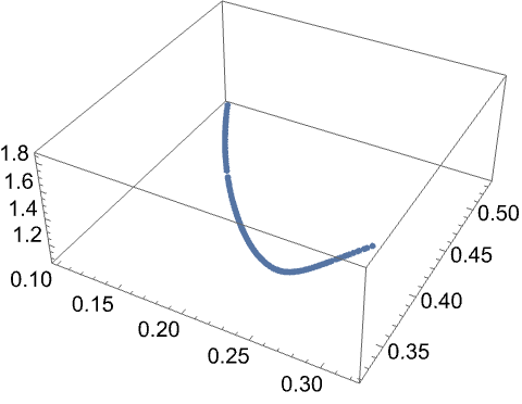 |
The solutions are then ranked by the ratio of the desired-to-leading-order error field harmonic magnitudes.
Specifying fewer field harmonics to be nulled results in a solution contour of higher dimensionality. Use three saddle primitives to null only one field harmonic, and the solution contour is a 2D surface embedded in a 3D space:
| In[13]:= |
| In[14]:= |
| Out[14]= | 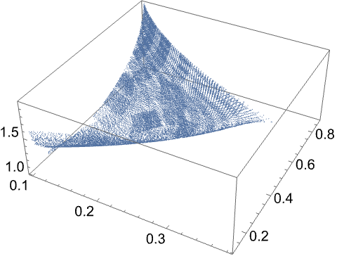 |
Although the interpolation algorithm works for arbitrary solution contour and search space dimensions, it is currently only optimised for a 1D solution contour (the default and most useful case).
Wolfram Language Version 13.0
Creative Commons Attribution Non Commercial 3.0 Unported