Resource retrieval
Get the pre-trained net:
NetModel parameters
This model consists of a family of individual nets, each identified by a specific parameter combination. Inspect the available parameters:
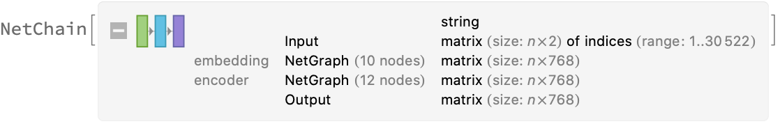
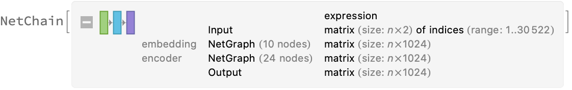
Pick a non-default net by specifying the parameters:
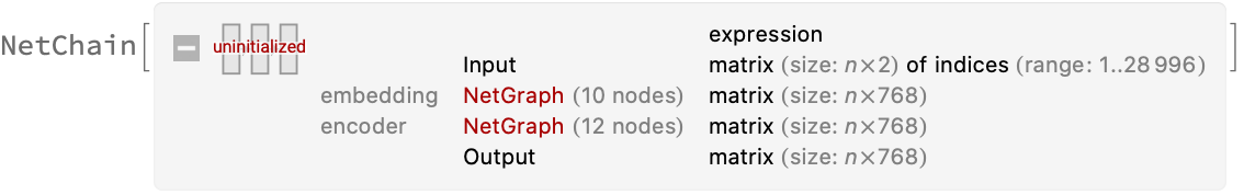
Pick a non-default uninitialized net:
Basic usage
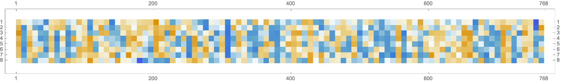
Given a piece of text, the BERT net produces a sequence of feature vectors of size 768, which corresponds to the sequence of input words or subwords:
Obtain dimensions of the embeddings:
Visualize the embeddings:
Transformer architecture
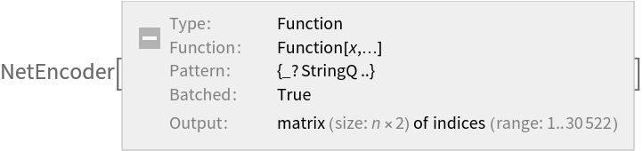
Each input text segment is first tokenized into words or subwords using a word-piece tokenizer and additional text normalization. Integer codes called token indices are generated from these tokens, together with additional segment indices:
For each input subword token, the encoder yields a pair of indices that corresponds to the token index in the vocabulary and the index of the sentence within the list of input sentences:
The list of tokens always starts with special token index 102, which corresponds to the classification index.
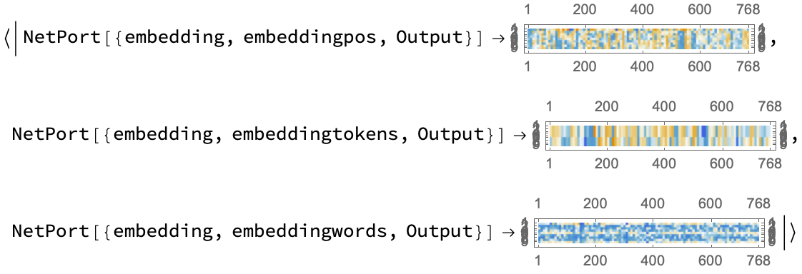
Also the special token index 103 is used as a separator between the different text segments. Each subword token is also assigned a positional index:
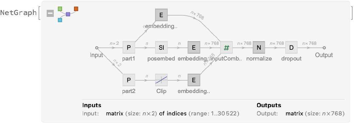
A lookup is done to map these indices to numeric vectors of size 768:
For each subword token, these three embeddings are combined by summing elements with ThreadingLayer:
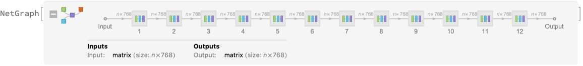
The transformer architecture then processes the vectors using 12 structurally identical self-attention blocks stacked in a chain:
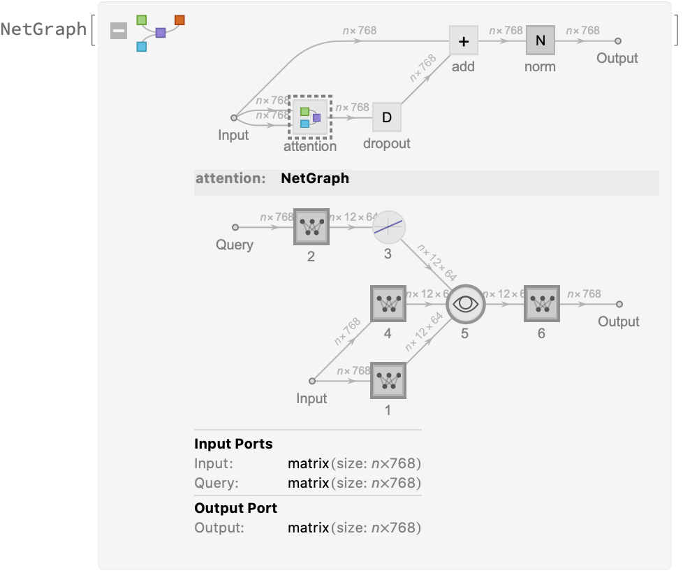
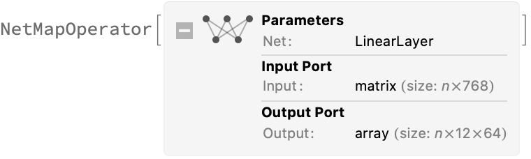
The key part of these blocks is the attention module comprising of 12 parallel self-attention transformations, also called “attention heads”:
Each head uses an AttentionLayer at its core:
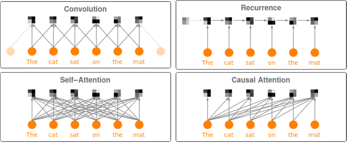
BERT uses self-attention, where the embedding of a given subword depends on the full input text. The following figure compares self-attention (lower left) to other types of connectivity patterns that are popular in deep learning:
Sentence analogies
Define a sentence embedding that takes the last feature vector from BERT subword embeddings (as an arbitrary choice):
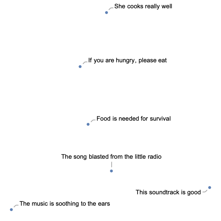
Define a list of sentences in two broad categories (food and music):
Precompute the embeddings for a list of sentences:
Visualize the similarity between the sentences using the net as a feature extractor:
Train a classifier model with the subword embeddings
Get a text-processing dataset:
View a random sample of the dataset:
Precompute the BERT vectors for the training and the validation datasets (if available, GPU is highly recommended):
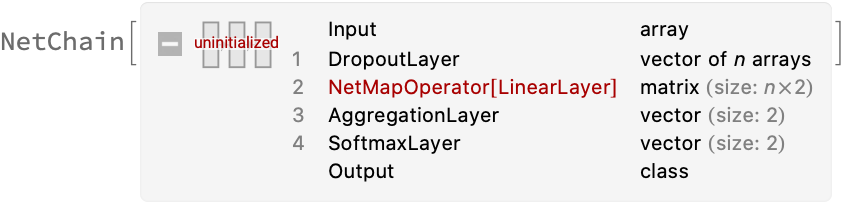
Define a network to classify the sequences of subword embeddings, using a max-pooling strategy:
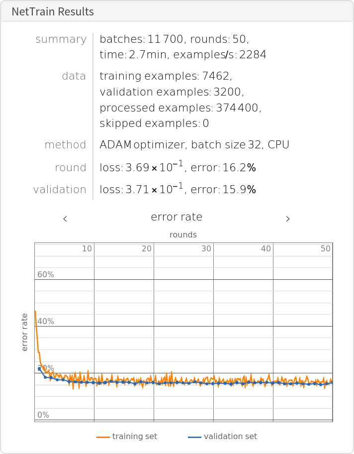
Train the network on the precomputed BERT vectors:
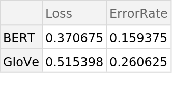
Check the classification error rate on the validation data:
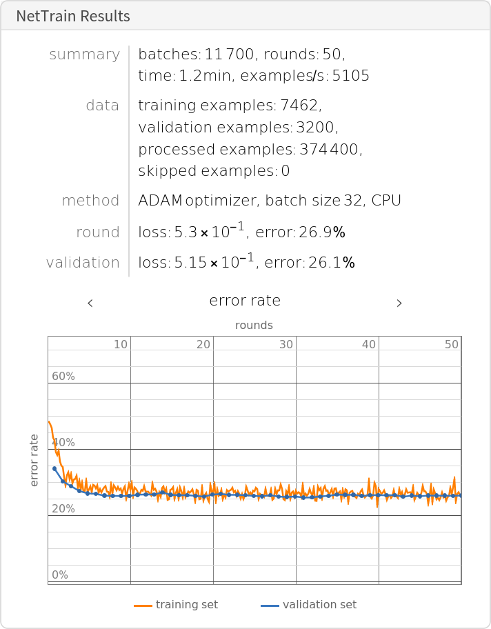
Let’s compare the results with the performance of a classifier trained on context-independent word embeddings. Precompute the GloVe vectors for the training and the validation dataset:
Train the classifier on the precomputed GloVe vectors:
Compare the results obtained with GPT and with GloVe:
Net information
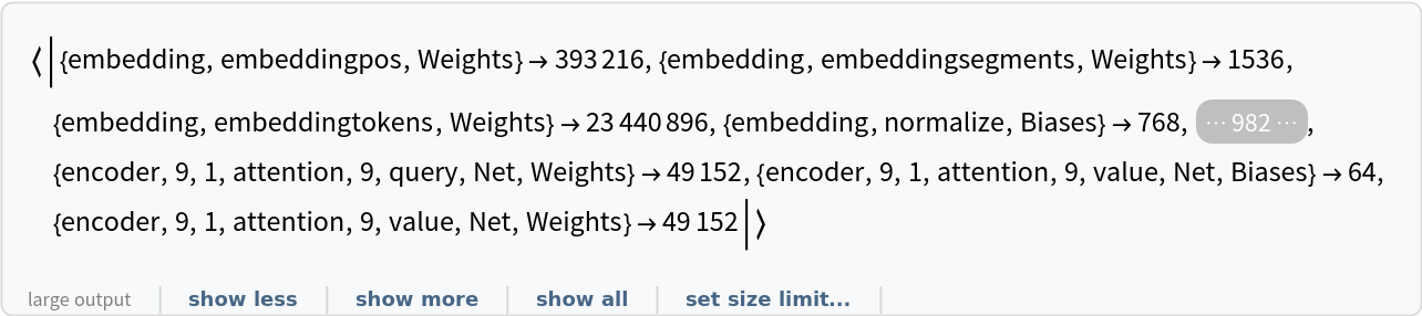
Inspect the number of parameters of all arrays in the net:
Obtain the total number of parameters:
Obtain the layer type counts:
Display the summary graphic:
Export to MXNet
Export the net into a format that can be opened in MXNet:
Export also creates a net.params file containing parameters:
Get the size of the parameter file:

![NetModel[{"BERT Trained on BookCorpus and Wikipedia Data", "Type" -> "LargeUncased", "InputType" -> "ListOfStrings"}]](https://www.wolframcloud.com/obj/resourcesystem/images/ea7/ea758ad7-0944-481e-a6a1-205ab1ac8a7d/44d5d605425fe237.png)
![NetModel[{"BERT Trained on BookCorpus and Wikipedia Data", "Type" -> "BaseCased", "InputType" -> "ListOfStrings"}, "UninitializedEvaluationNet"]](https://www.wolframcloud.com/obj/resourcesystem/images/ea7/ea758ad7-0944-481e-a6a1-205ab1ac8a7d/26080a608386308d.png)
![net = NetModel[{"BERT Trained on BookCorpus and Wikipedia Data", "InputType" -> "ListOfStrings"}];
netencoder = NetExtract[net, "Input"]](https://www.wolframcloud.com/obj/resourcesystem/images/ea7/ea758ad7-0944-481e-a6a1-205ab1ac8a7d/25a8594f3f2b89ff.png)
![embeddings = net[{"Hello world!", "I am here"},
{NetPort[{"embedding", "embeddingpos", "Output"}],
NetPort[{"embedding", "embeddingtokens", "Output"}],
NetPort[{"embedding", "embeddingwords", "Output"}]}];
Map[MatrixPlot, embeddings]](https://www.wolframcloud.com/obj/resourcesystem/images/ea7/ea758ad7-0944-481e-a6a1-205ab1ac8a7d/08eae81f0b1bea8b.png)
![sentenceembedding = NetAppend[NetModel["BERT Trained on BookCorpus and Wikipedia Data"], "pooling" -> SequenceLastLayer[]]](https://www.wolframcloud.com/obj/resourcesystem/images/ea7/ea758ad7-0944-481e-a6a1-205ab1ac8a7d/5d02a8dda1528c9e.png)

![train = ResourceData["Sample Data: Movie Review Sentence Polarity", "TrainingData"];
valid = ResourceData["Sample Data: Movie Review Sentence Polarity", "TestData"];](https://www.wolframcloud.com/obj/resourcesystem/images/ea7/ea758ad7-0944-481e-a6a1-205ab1ac8a7d/7a9841a183d94324.png)
![trainembeddings = NetModel["BERT Trained on BookCorpus and Wikipedia Data"][
train[[All, 1]], TargetDevice -> "CPU"] -> train[[All, 2]];
validembeddings = NetModel["BERT Trained on BookCorpus and Wikipedia Data"][
valid[[All, 1]], TargetDevice -> "CPU"] -> valid[[All, 2]];](https://www.wolframcloud.com/obj/resourcesystem/images/ea7/ea758ad7-0944-481e-a6a1-205ab1ac8a7d/68d961b3bba79b9e.png)
![classifierhead = NetChain[{DropoutLayer[], NetMapOperator[2], AggregationLayer[Max, 1], SoftmaxLayer[]}, "Output" -> NetDecoder[{"Class", {"negative", "positive"}}]]](https://www.wolframcloud.com/obj/resourcesystem/images/ea7/ea758ad7-0944-481e-a6a1-205ab1ac8a7d/75e6e147f3355989.png)
![bertresults = NetTrain[classifierhead, trainembeddings, All,
ValidationSet -> validembeddings,
TargetDevice -> "CPU",
MaxTrainingRounds -> 50]](https://www.wolframcloud.com/obj/resourcesystem/images/ea7/ea758ad7-0944-481e-a6a1-205ab1ac8a7d/407342886ed5b257.png)
![trainembeddingsglove = NetModel[
"GloVe 300-Dimensional Word Vectors Trained on Wikipedia and Gigaword 5 Data"][train[[All, 1]], TargetDevice -> "CPU"] -> train[[All, 2]];
validembeddingsglove = NetModel[
"GloVe 300-Dimensional Word Vectors Trained on Wikipedia and Gigaword 5 Data"][valid[[All, 1]], TargetDevice -> "CPU"] -> valid[[All, 2]];](https://www.wolframcloud.com/obj/resourcesystem/images/ea7/ea758ad7-0944-481e-a6a1-205ab1ac8a7d/4fe0a4523cf29883.png)
![gloveresults = NetTrain[classifierhead, trainembeddingsglove, All,
ValidationSet -> validembeddingsglove,
TrainingStoppingCriterion -> <|"Criterion" -> "ErrorRate", "Patience" -> 50|>,
TargetDevice -> "CPU",
MaxTrainingRounds -> 50]](https://www.wolframcloud.com/obj/resourcesystem/images/ea7/ea758ad7-0944-481e-a6a1-205ab1ac8a7d/6539b466f0befba0.png)
![NetInformation[
NetModel[
"BERT Trained on BookCorpus and Wikipedia Data"], "ArraysElementCounts"]](https://www.wolframcloud.com/obj/resourcesystem/images/ea7/ea758ad7-0944-481e-a6a1-205ab1ac8a7d/3d608357398d72d2.png)
![NetInformation[
NetModel[
"BERT Trained on BookCorpus and Wikipedia Data"], "ArraysTotalElementCount"]](https://www.wolframcloud.com/obj/resourcesystem/images/ea7/ea758ad7-0944-481e-a6a1-205ab1ac8a7d/7a43df2d69d2200c.png)

![jsonPath = Export[FileNameJoin[{$TemporaryDirectory, "net.json"}], NetModel["BERT Trained on BookCorpus and Wikipedia Data"], "MXNet"]](https://www.wolframcloud.com/obj/resourcesystem/images/ea7/ea758ad7-0944-481e-a6a1-205ab1ac8a7d/346c4453073b77b6.png)