Resource retrieval
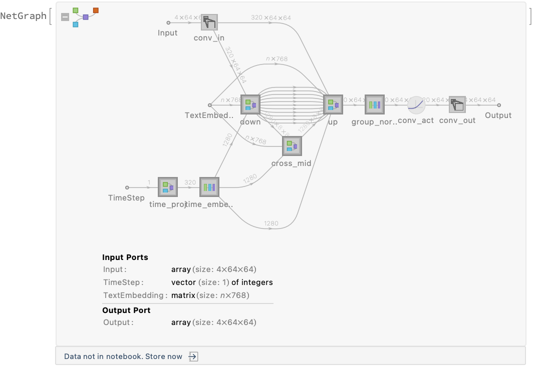
Get the pre-trained net:
NetModel parameters
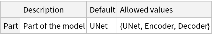
This model consists of a family of individual nets, each identified by a specific parameter combination. Inspect the available parameters:
Pick a non-default net by specifying the parameters:
Pick a non-default uninitialized net:
Evaluation function
Write an evaluation function to automate the image generation:
Basic usage
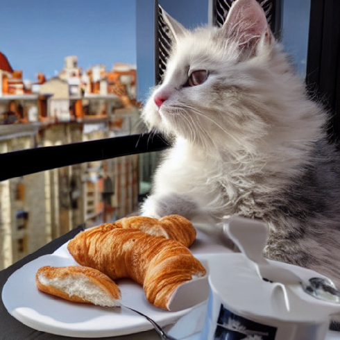
Define a test prompt:
Generate an image based on the test prompt:
Define the guidance scale, which by default is set to 7.5, and regenerate the image. Lowering the guidance scale can lead to generated outputs that deviate further from the specified prompt and may introduce excessive randomness, resulting in less fidelity to the desired characteristics:
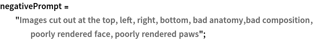
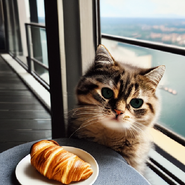
The negative prompt is used to address specific issues or challenges in generating desired images. By providing a negative prompt, it allows the model to focus on avoiding or minimizing certain undesired features or qualities in the generated image. Define the negative prompt and recreate an image:
The reference image is used to guide the model in generating images with a desired style or with desired attributes. Recreate an image by utilizing the negative prompt and the reference image, allowing the diffusion process to progress through 90% of its steps:
Please note that even when the negative prompt is used, it may not guarantee the resolution of all the problems:
Possible issues
Using a guidance scale smaller than 1 (classifier-free guidance) might not produce a meaningful result:
Note that using the same text for both the prompt and negative prompt results in an identical outcome to the classifier-free guidance. However, this approach takes twice as long in terms of processing time:
Visualize backward diffusion
Define the prompt and the negative prompt:
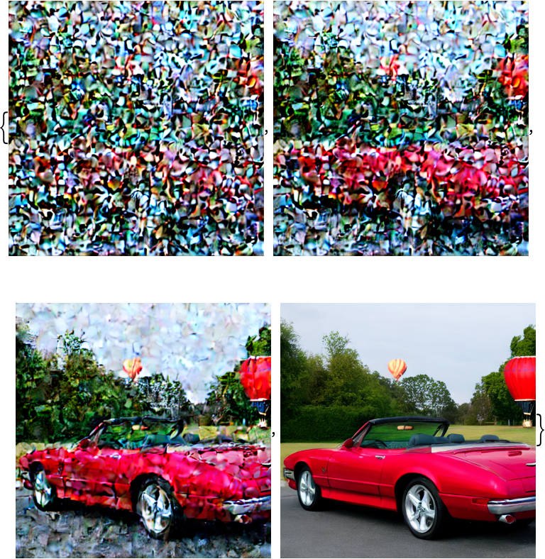
Visualize the backward diffusion at intervals of 25% of the generation process:
Variational autoencoder
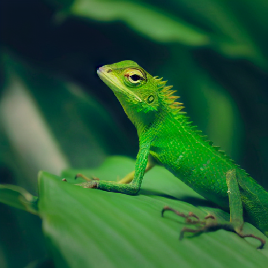
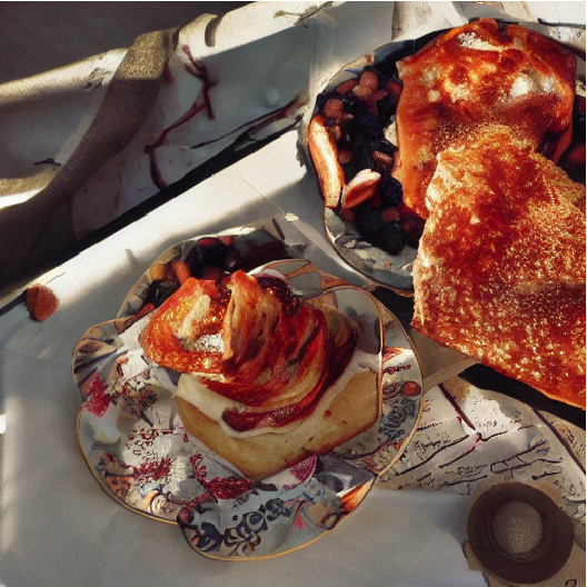
Define a test image:
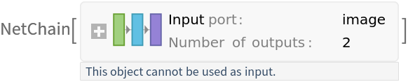
In the Stable Diffusion training pipeline, the encoder is responsible for encoding the reference image into a low-dimensional latent representation, which will serve as the input for the U-Net model. After the training, it is not used for generating images. Get the variational autoencoder (VAE) encoder:
Encode the test image to obtain the mean and variance of the latent space distribution conditioned on the input image:
The distribution mean can be interpreted as a compressed version of the image. Calculate the compression ratio:
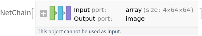
In the Stable Diffusion pipeline, the denoised latent representations generated through the reverse diffusion process are transformed back into images using the VAE decoder. Get the VAE decoder:
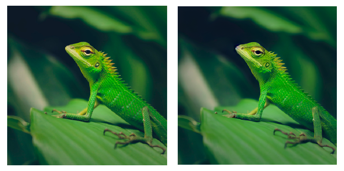
Decode the result to reconstruct the image by choosing the mean of the posterior distribution:
Compare the results:
Net information
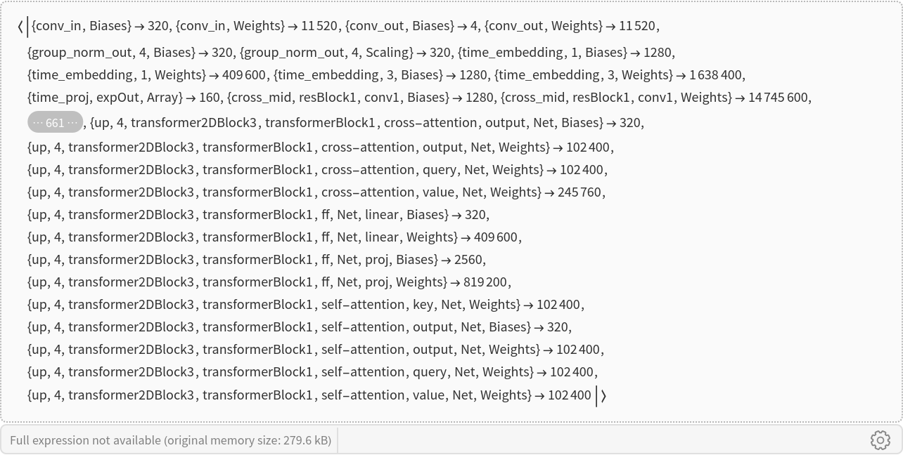
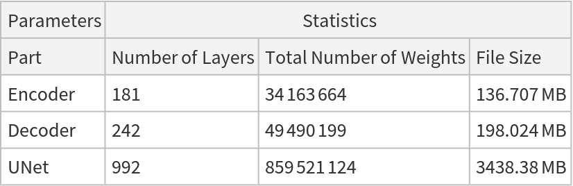
Inspect the number of parameters of all arrays in the net:
Obtain the total number of parameters:
Obtain the layer type counts:
![(* Evaluate this cell to get the example input *) CloudGet["https://www.wolframcloud.com/obj/56e2e139-7e1a-4568-8225-d4174bcf71d2"]](https://www.wolframcloud.com/obj/resourcesystem/images/e38/e3849c24-360b-43a5-a8c8-e32ea5f89140/7492430e0283e554.png)

![(* Evaluate this cell to get the example input *) CloudGet["https://www.wolframcloud.com/obj/f8238ede-4392-44ea-8e2b-366848205b3a"]](https://www.wolframcloud.com/obj/resourcesystem/images/e38/e3849c24-360b-43a5-a8c8-e32ea5f89140/6250f53f71908485.png)
![netEvaluate[<|
"Prompt" -> prompt, "NegativePrompt" -> negativePrompt
|>]](https://www.wolframcloud.com/obj/resourcesystem/images/e38/e3849c24-360b-43a5-a8c8-e32ea5f89140/473c0ba1cb298ada.png)
![netEvaluate[<|
"Prompt" -> newPrompt, "NegativePrompt" -> newNegativePrompt,
"Image" -> (img -> diffusionStrength)
|>]](https://www.wolframcloud.com/obj/resourcesystem/images/e38/e3849c24-360b-43a5-a8c8-e32ea5f89140/6e89714bb4bf5cdd.png)
![(* Evaluate this cell to get the example input *) CloudGet["https://www.wolframcloud.com/obj/7f4d9124-9c73-4ae0-a368-ab8a9a8c22ce"]](https://www.wolframcloud.com/obj/resourcesystem/images/e38/e3849c24-360b-43a5-a8c8-e32ea5f89140/6e75c1417517c98e.png)
![netEvaluate[
<|"Prompt" -> (prompt -> 0)|>,
MaxIterations -> 20,
RandomSeeding -> 1234
]](https://www.wolframcloud.com/obj/resourcesystem/images/e38/e3849c24-360b-43a5-a8c8-e32ea5f89140/186cc290914c6a9e.png)
![netEvaluate[
<|
"Prompt" -> prompt, "NegativePrompt" -> prompt
|>,
MaxIterations -> 20,
RandomSeeding -> 1234
]](https://www.wolframcloud.com/obj/resourcesystem/images/e38/e3849c24-360b-43a5-a8c8-e32ea5f89140/41f7e0366b48f9c3.png)

![(* Evaluate this cell to get the example input *) CloudGet["https://www.wolframcloud.com/obj/49ac9611-eae9-4264-81e5-147fa233bbd4"]](https://www.wolframcloud.com/obj/resourcesystem/images/e38/e3849c24-360b-43a5-a8c8-e32ea5f89140/1c84226167122025.png)
![inputSize = Times @@ NetExtract[
NetModel["Stable Diffusion V1", "Part" -> "Encoder"], {"Input", "Output"}];
outputSize = Times @@ Dimensions[encoded["Mean"]];
N[outputSize/inputSize]](https://www.wolframcloud.com/obj/resourcesystem/images/e38/e3849c24-360b-43a5-a8c8-e32ea5f89140/6557274a20bae07b.png)