Resource retrieval

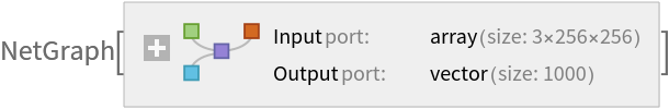
Get the pre-trained net:

In[1]:=

Out[1]=

NetModel parameters

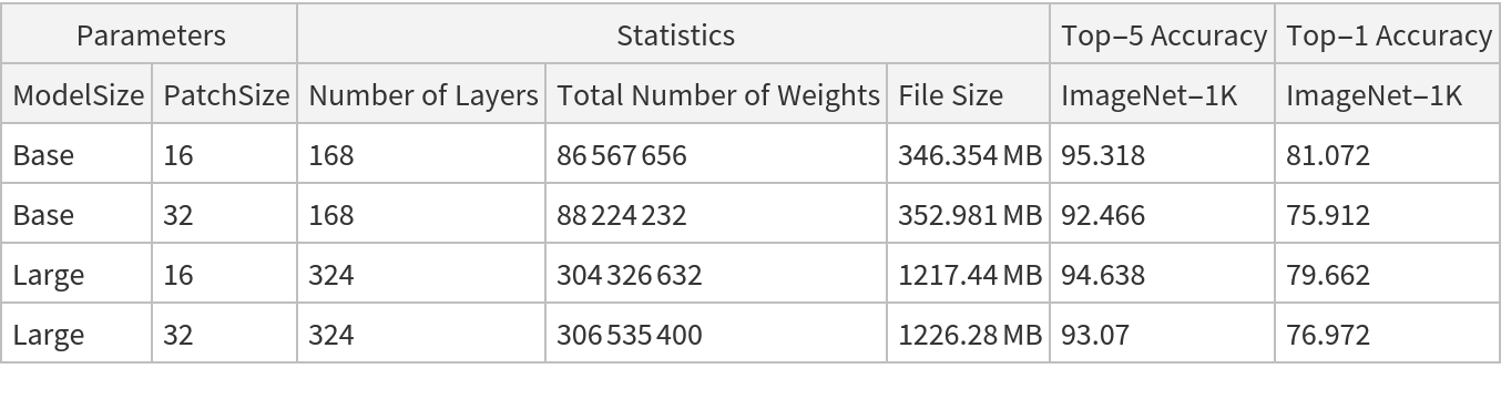
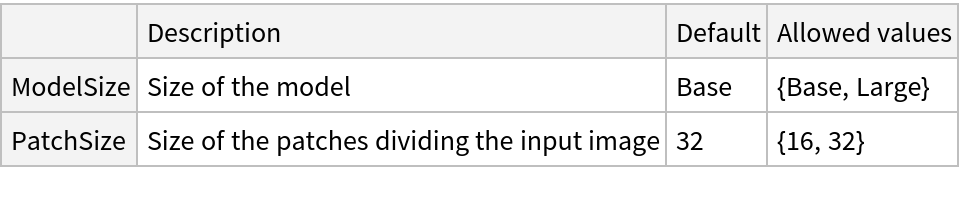
This model consists of a family of individual nets, each identified by a specific parameter combination. Inspect the available parameters:

In[2]:=

Out[2]=

Pick a non-default net by specifying the parameters:

In[3]:=

Out[3]=

Pick a non-default uninitialized net:

In[4]:=

Out[4]=

Basic usage

Classify an image:

In[5]:=

Out[5]=

The prediction is an Entity object, which can be queried:

In[6]:=

Out[6]=

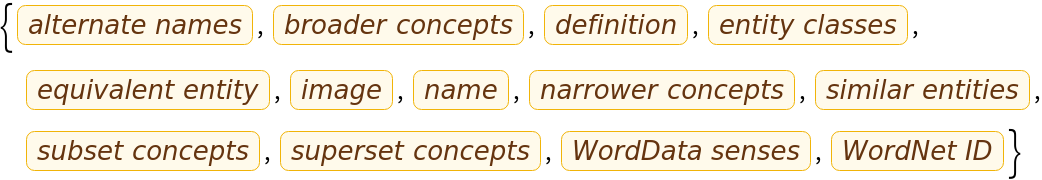
Get the list of available properties for the predicted Entity:

In[7]:=

Out[7]=

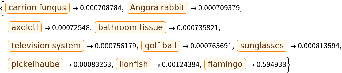
Obtain the probabilities of the 10 most likely entities predicted by the net. Note that the top 10 predictions are not mutually exclusive:

In[8]:=

Out[8]=

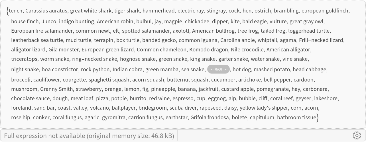
Obtain the list of names of all available classes:

In[9]:=

Out[9]=

Net architecture

The main idea behind this vision transformer is to divide the input image into a grid of 7x7 patches, represent each part as a feature vector and perform self-attention on such set of 49 feature vectors, or "tokens." One additional feature vector is used as the "classification token," which will contain the class information at the end of the processing.

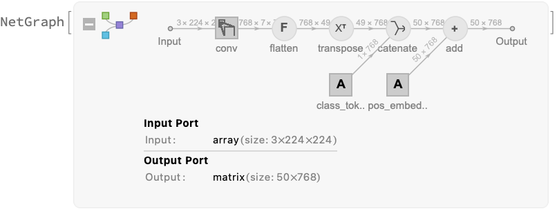
After extracting the pixel values and taking a center crop of the image, the first module of the net computes the initial values for the set of 50 "tokens":

In[10]:=

Out[10]=

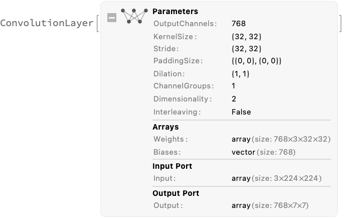
The patches are computed using the only ConvolutionLayer in the net. It takes the center crop and produces 7x7 patches with feature size 768. Each of the 49 patches represents a 32x32 area on the original image:

In[11]:=

Out[11]=

The patches are then reshaped and transposed to an array of shape 49x768, so that each patch is encoded into a feature vector of size 768. Then the "classification token" is prepended (bringing the vector count to 50), after which the positional embeddings are added to each vector:

In[12]:=

In[13]:=

Out[13]=

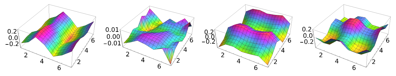
Positional embeddings are added to the input image patches to add some notion of spatial awareness to the downstream attention processing. Just like most sequence-based transformers for NLP, the values of the embeddings for fixed feature dimensions often exhibit an oscillating structure, except this time they vary along two dimensions. Inspect a few positional embeddings for different features:

In[14]:=

In[15]:=

Out[15]=

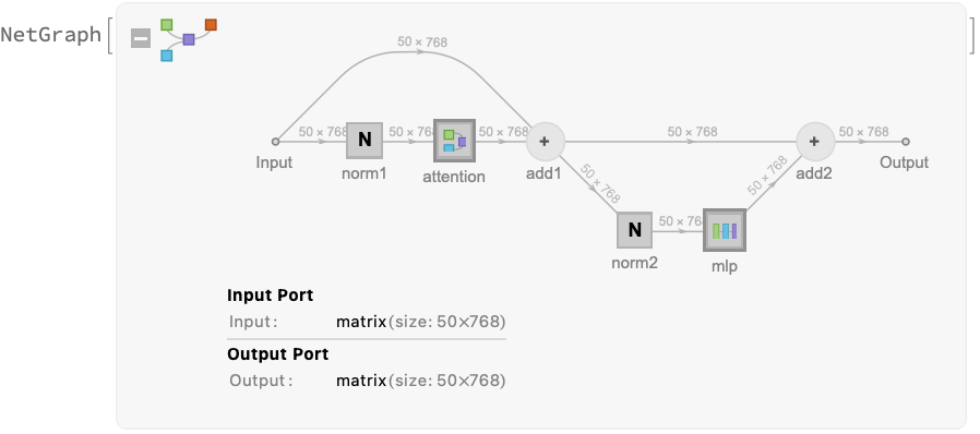
After adding the positional embeddings, the sequence of 50 vectors is fed to a stack of 12 structurally identical self-attention blocks, consisting of a self-attention part and a simple MLP part:

In[16]:=

Out[16]=

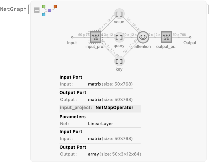
The self-attention part is a standard multi-head attention setup. The feature size 768 is divided into 12 heads each with size 64:

In[17]:=

Out[17]=

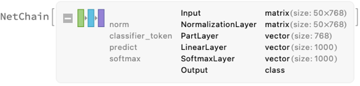
After the self-attention stack, the set of vectors is normalized one last time and the "classification token" is extracted and used to classify the image:

In[18]:=

Out[18]=

Attention visualization

Define a test image and classify it:

In[19]:=

In[20]:=

Out[20]=

Extract the attention weights used for the last block of self-attention when classifying this image:

In[21]:=

In[22]:=

Out[22]=

Extract the attention weights between the "classification token" and the input patches. These weights can be interpreted as which patches in the original image the net is "looked at" in order to perform the classification:

In[23]:=

Out[24]=

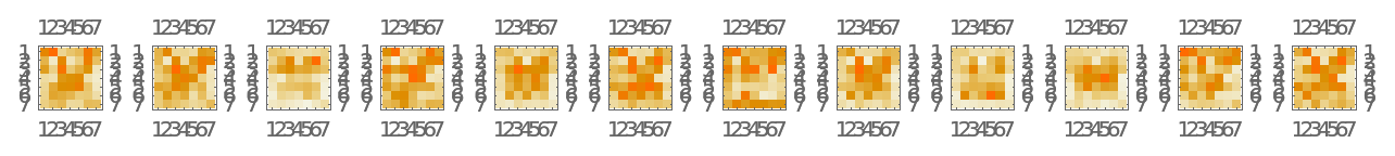
Reshape the weights as a 3D array of 12 7x7 matrices. Each matrix corresponds to a head, while each element of the matrices corresponds to a patch in the original image:

In[25]:=

Visualize the attention weight matrices. Patches with higher values (red color) are what is mostly being "looked at" for each attention head:

In[26]:=

Out[26]=

Define a function to visualize the attention matrix on an image:

In[27]:=

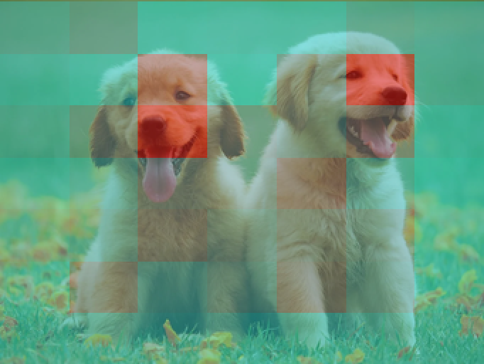
Visualize the mean attention across all the attention heads:

In[28]:=

Out[28]=

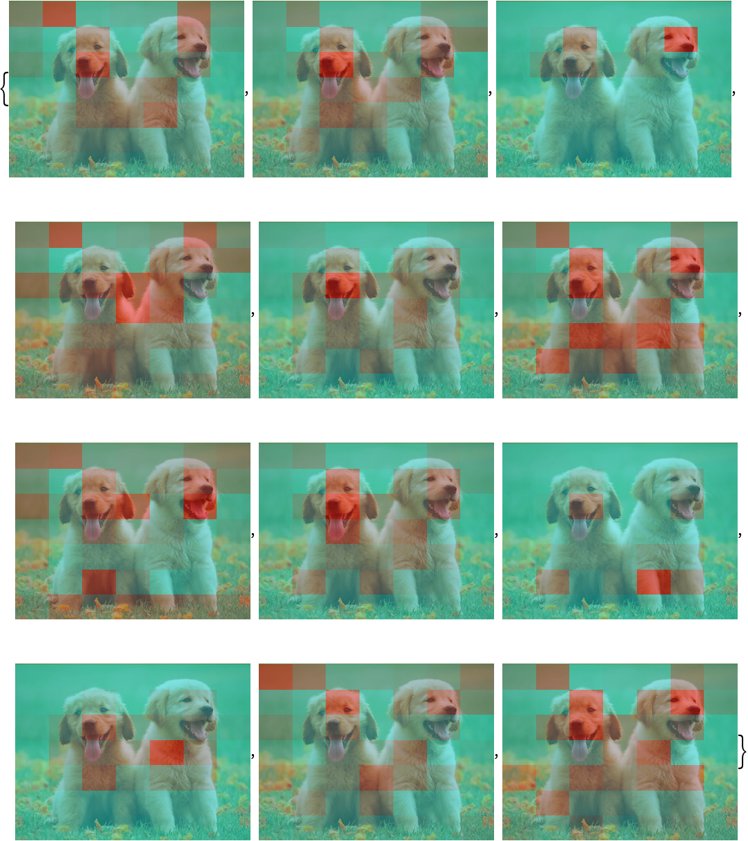
Visualize each attention head separately:

In[29]:=

Out[29]=

Positional embedding visualization

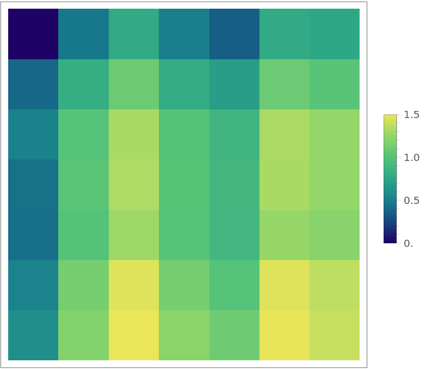
Positional embeddings for spatially distant patches tend to be apart in the feature space as well. In order to show this, calculate the distance matrix between the embeddings of the input patches:

In[30]:=

In[31]:=

In[32]:=

Out[32]=

Visualize the distance between all patches and the first (top-left) patch:

In[33]:=

In[34]:=

Out[34]=

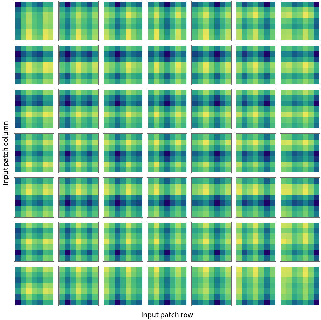
Repeat the experiment for all the patches. Note that patches in the same row or column are closer to each other:

In[35]:=

In[36]:=

Out[36]=

Feature extraction

Remove the last two layers of the trained net so that the net produces a vector representation of an image:

In[37]:=

Out[37]=

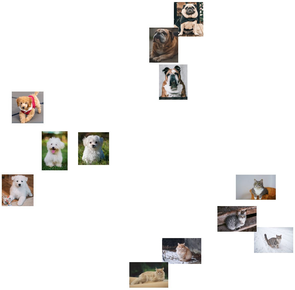
Get a set of images:

In[38]:=

Visualize the features of a set of images:

In[39]:=

Out[39]=

Transfer learning

Use the pre-trained model to build a classifier for telling apart indoor and outdoor photos. Create a test set and a training set:

In[40]:=

In[41]:=

Remove the last linear layer from the pre-trained net:

In[42]:=

Out[42]=

Create a new net composed of the pre-trained net followed by a linear layer and a softmax layer:

In[43]:=

Train on the dataset, freezing all the weights except for those in the "linearNew" layer (use TargetDevice -> "GPU" for training on a GPU):

In[44]:=

Out[44]=

Perfect accuracy is obtained on the test set:

In[45]:=

Out[45]=

Net information

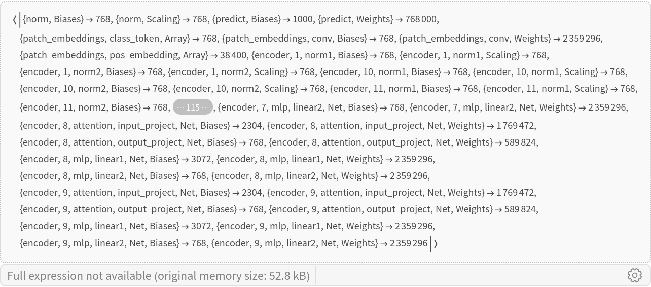
Inspect the number of parameters of all arrays in the net:

In[46]:=

Out[46]=

Obtain the total number of parameters:

In[47]:=

Out[47]=

Obtain the layer type counts:

In[48]:=

Out[48]=

Export to ONNX

Export the net to the ONNX format:

In[49]:=

Out[49]=

Get the size of the ONNX file:

In[50]:=

Out[50]=

Check some metadata of the ONNX model:

In[51]:=

Out[51]=

Import the model back into Wolfram Language. However, the NetEncoder and NetDecoder will be absent because they are not supported by ONNX:

In[52]:=

Out[52]=