Ademxapp Model A1
Trained on
ADE20K Data
Released in 2016 by the University of Adelaide, this model exploits recent progress in the understanding of residual architectures. With only 17 residual units, it is able to outperform previous, much deeper architectures.
Number of layers: 141 |
Parameter count: 124,684,886 |
Trained size: 499 MB |
Examples
Resource retrieval
Get the pre-trained net:
Evaluation function
Write an evaluation function to handle net reshaping and resampling of input and output:
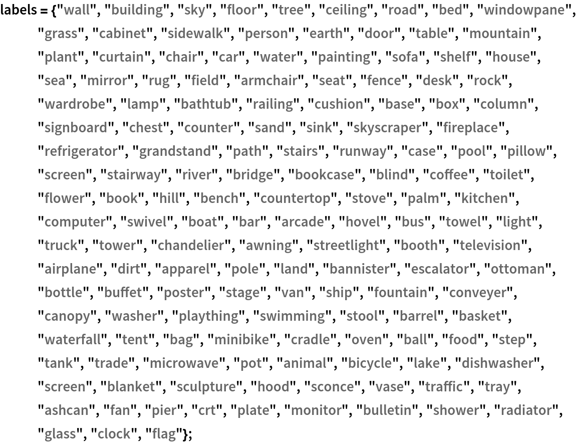
Label list
Define the label list for this model. Integers in the model’s output correspond to elements in the label list:
Basic usage
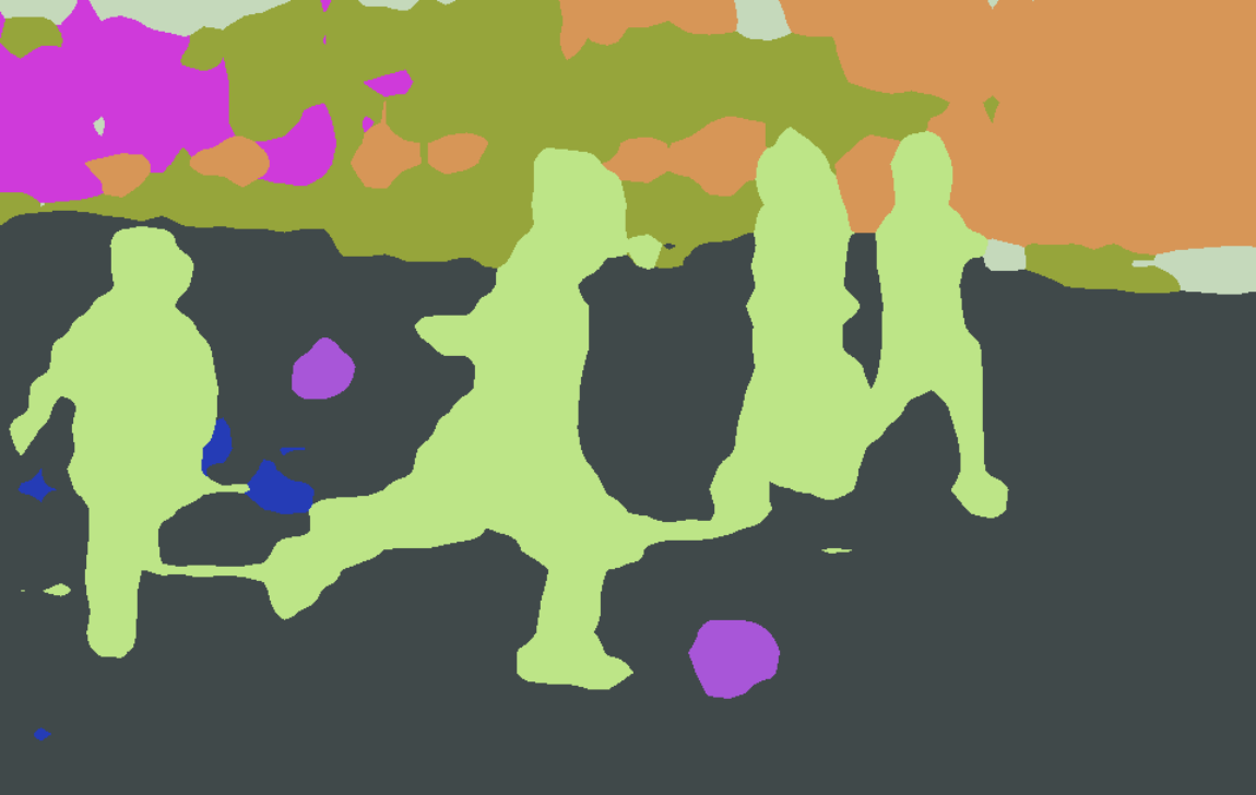
Obtain a segmentation mask for a given image:
Inspect which classes are detected:
Visualize the mask:
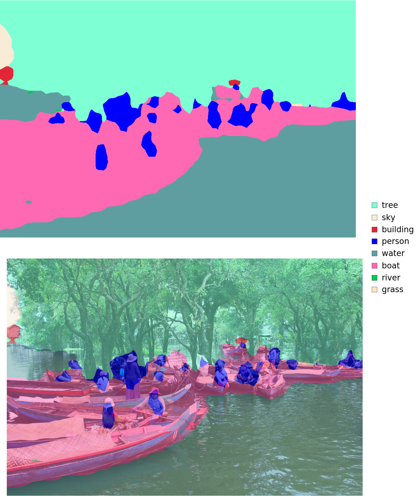
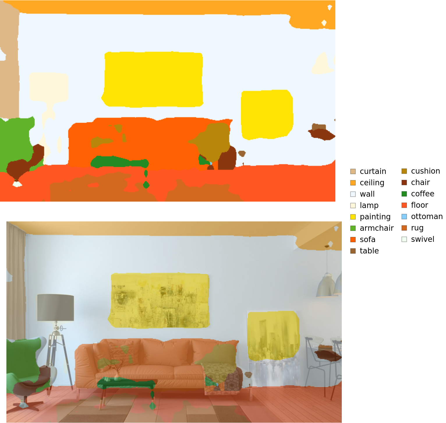
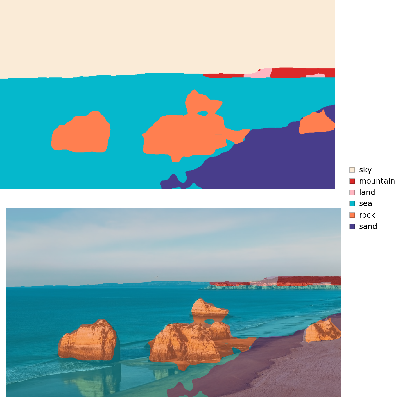
Advanced visualization
Associate classes to colors:
Write a function to overlap the image and the mask with a legend:
Inspect the results:
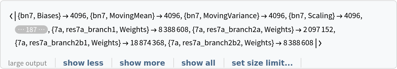
Net information
Inspect the sizes of all arrays in the net:
Obtain the total number of parameters:
Obtain the layer type counts:
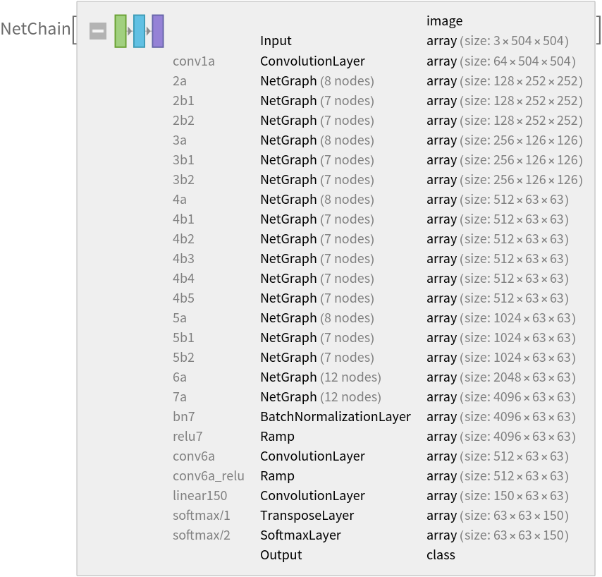
Display the summary graphic:
Export to MXNet
Export the net into a format that can be opened in MXNet:
Export also creates a net.params file containing parameters:
Get the size of the parameter file:
The size is similar to the byte count of the resource object:
Requirements
Wolfram Language
11.3
(March 2018)
or above
Resource History
Reference
![netevaluate[img_, device_ : "CPU"] := Block[
{net, resized, encData, dec, mean, var, prob},
net = NetModel["Ademxapp Model A1 Trained on ADE20K Data"];
resized = ImageResize[img, {504}];
encData = Normal@NetExtract[net, "Input"];
dec = NetExtract[net, "Output"];
{mean, var} = Lookup[encData, {"MeanImage", "VarianceImage"}];
prob = NetReplacePart[net,
{"Input" -> NetEncoder[{"Image", ImageDimensions@resized, "MeanImage" -> mean, "VarianceImage" -> var}], "Output" -> Automatic}
][resized, TargetDevice -> device];
prob = ArrayResample[prob, Append[Reverse@ImageDimensions@img, 150]];
dec[prob]
]](https://www.wolframcloud.com/obj/resourcesystem/images/b4b/b4b767a5-9c86-4f48-a6b3-0cd78be1bf2e/685185797edb5d7a.png)
![(* Evaluate this cell to get the example input *) CloudGet["https://www.wolframcloud.com/obj/44352668-c413-4c3f-8394-5b90298e01d3"]](https://www.wolframcloud.com/obj/resourcesystem/images/b4b/b4b767a5-9c86-4f48-a6b3-0cd78be1bf2e/7733656d83d36502.png)
![result[img_, device_ : "CPU"] := Block[
{mask, classes, maskPlot, composition},
mask = netevaluate[img, device];
classes = DeleteDuplicates[Flatten@mask];
maskPlot = Colorize[mask, ColorRules -> indexToColor];
composition = ImageCompose[img, {maskPlot, 0.5}];
Legended[
Row[Image[#, ImageSize -> Large] & /@ {maskPlot, composition}], SwatchLegend[indexToColor[[classes, 2]], labels[[classes]]]]
]](https://www.wolframcloud.com/obj/resourcesystem/images/b4b/b4b767a5-9c86-4f48-a6b3-0cd78be1bf2e/6c7857a8ded30b98.png)
![(* Evaluate this cell to get the example input *) CloudGet["https://www.wolframcloud.com/obj/65a16927-e2bd-4f93-81a7-6a1f8a8adb9c"]](https://www.wolframcloud.com/obj/resourcesystem/images/b4b/b4b767a5-9c86-4f48-a6b3-0cd78be1bf2e/1c5dd092bed86bfc.png)
![(* Evaluate this cell to get the example input *) CloudGet["https://www.wolframcloud.com/obj/86603e02-9d75-49bb-83e0-e01abbbc8425"]](https://www.wolframcloud.com/obj/resourcesystem/images/b4b/b4b767a5-9c86-4f48-a6b3-0cd78be1bf2e/1399059eb197b0e9.png)
![(* Evaluate this cell to get the example input *) CloudGet["https://www.wolframcloud.com/obj/033fb24b-0e5b-41e1-ae0d-14cc5bb0dec2"]](https://www.wolframcloud.com/obj/resourcesystem/images/b4b/b4b767a5-9c86-4f48-a6b3-0cd78be1bf2e/28c645e8dd726a33.png)