Resource retrieval
Get the pre-trained net:
NetModel parameters
This model consists of a family of individual nets, each identified by a specific parameter combination. Inspect the available parameters:
Pick a non-default net by specifying the parameters:
Pick a non-default uninitialized net:
Evaluation function
Define the label list for this model:
Define helper utilities for netevaluate:
Write an evaluation function to estimate the locations of the objects and human keypoints:
Basic usage
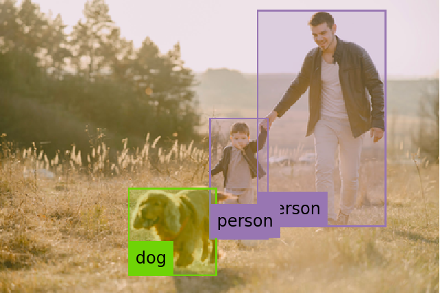
Obtain the detected bounding boxes with their corresponding classes and confidences as well as the locations of human joints for a given image:
Inspect the prediction keys:
The "ObjectDetection" key contains the coordinates of the detected objects as well as its confidences and classes:
Inspect which classes are detected:
The "KeypointEstimation" key contains the locations of top predicted keypoints as well as their confidences for each person:
Inspect the predicted keypoint locations:
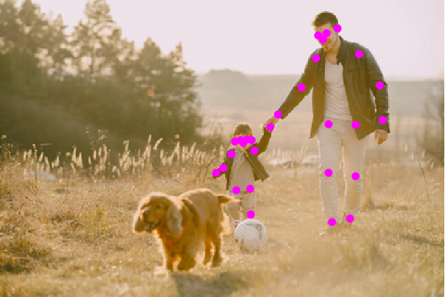
Visualize the keypoints:
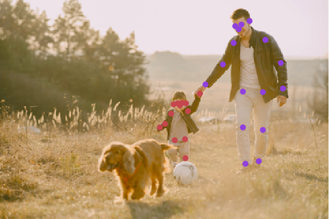
Visualize the keypoints grouped by person:
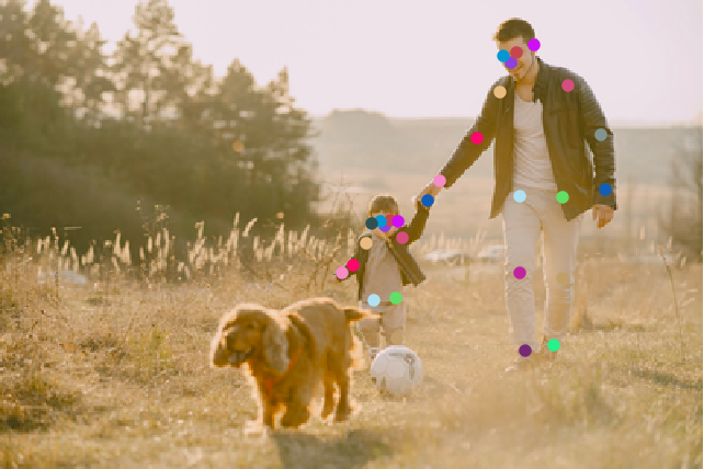
Visualize the keypoints grouped by a keypoint type:
Define a function to combine the keypoints into a skeleton shape:
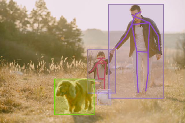
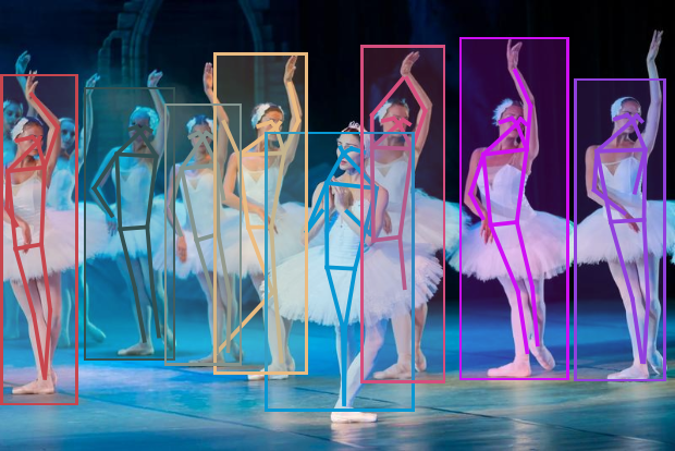
Visualize the pose keypoints, object detections and human skeletons:
Advanced visualization
Obtain the detected bounding boxes with their corresponding classes and confidences as well as the locations of human joints for a given image:
Visualize the pose keypoints, object detections and human skeletons. Note that some of the keypoints are misaligned:
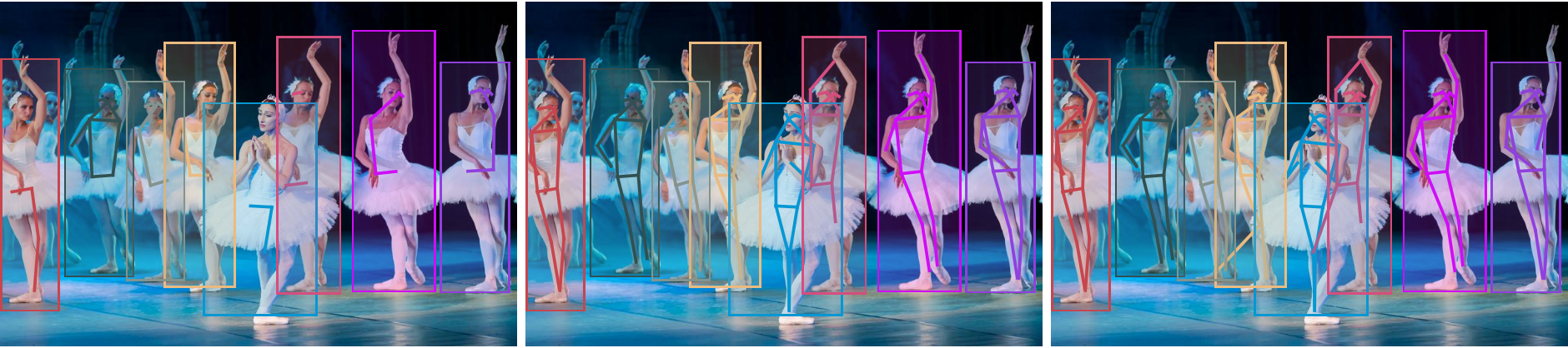
Inspect the various effects of a radius defined by an optional parameter "NeighborhoodRadius":
Network object detection result
For the default input size of 512x512, the net produces 128x128 bounding boxes whose centers mostly follow a square grid. For each bounding box, the net produces the box size and the offset of the box center with respect to the square grid:
Change the coordinate system into a graphics domain:
Compute and visualize the box center positions:
Visualize the box center positions. They follow a square grid with offsets:
Compute the boxes' coordinates:
Define a function to rescale the box coordinates to the original image size:
Visualize all the boxes predicted by the net scaled by their "objectness" measures:
Visualize all the boxes scaled by the probability that they contain a dog:
Superimpose the cat prediction on top of the scaled input received by the net:
Heat map visualization
Every box is associated to a scalar strength value indicating the likelihood that the patch contains an object:
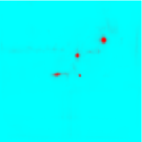
The strength of each patch is the maximal element aggregated across all classes. Obtain the strength of each patch:
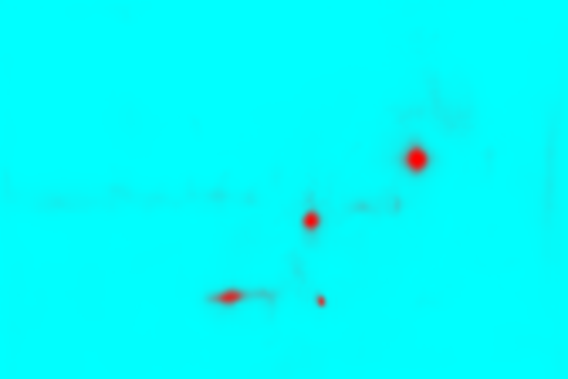
Visualize the strength of each patch as a heat map:
Stretch and unpad the heat map to the original image domain:
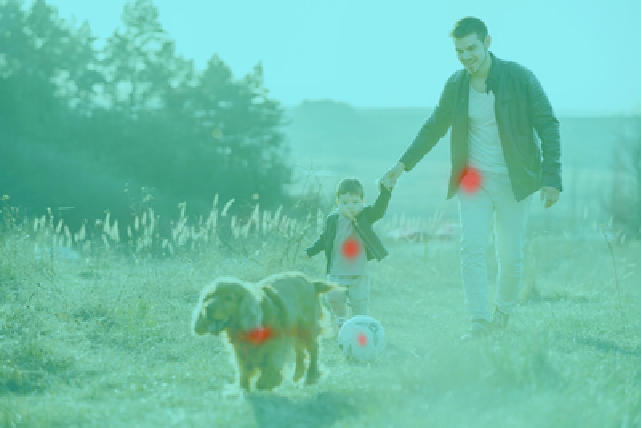
Overlay the heat map on the image:
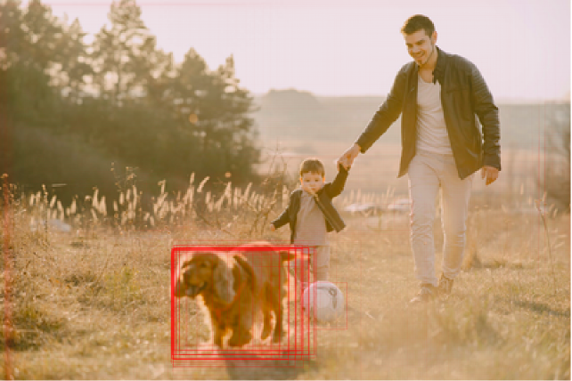
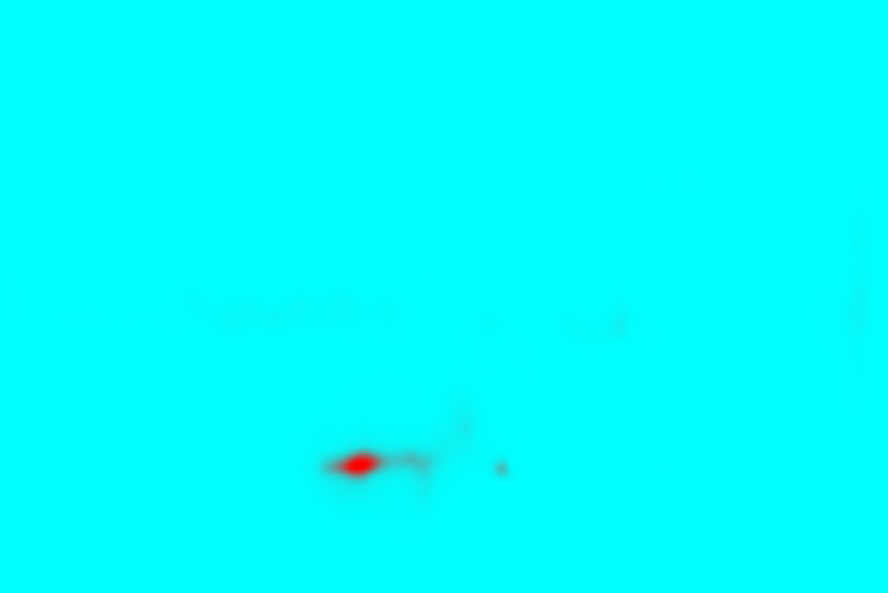
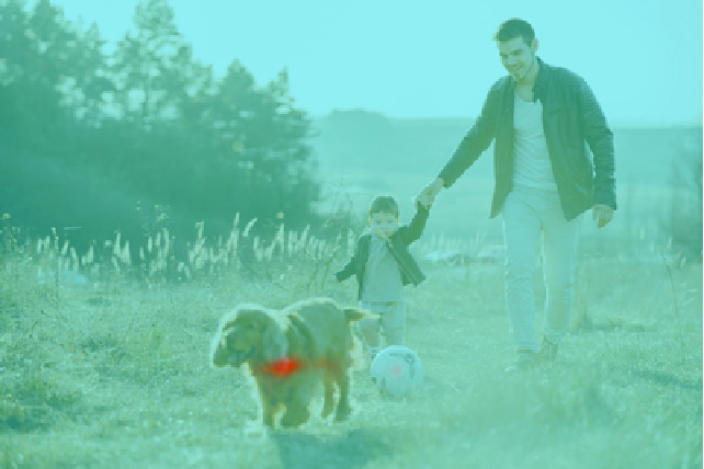
Obtain and visualize the strength of each patch for the "dog" class:
Overlay the heat map on the image:
Define a general function to visualize a heat map on an image:
Adapt to any size
Automatic image resizing can be avoided by replacing the NetEncoder. First get the NetEncoder:
Note that the NetEncoder resizes the image by keeping the aspect ratio and then pads the result to have a fixed shape of 512x512. Visualize the output of NetEncoder adjusting for brightness:
Create a new NetEncoder with the desired dimensions:
Attach the new NetEncoder:
Obtain the detected bounding boxes with their corresponding classes and confidences for a given image:
Visualize the detection:
Note that even though the localization results and the box confidences are slightly worse compared to the original net, the resized network runs significantly faster:
Net information
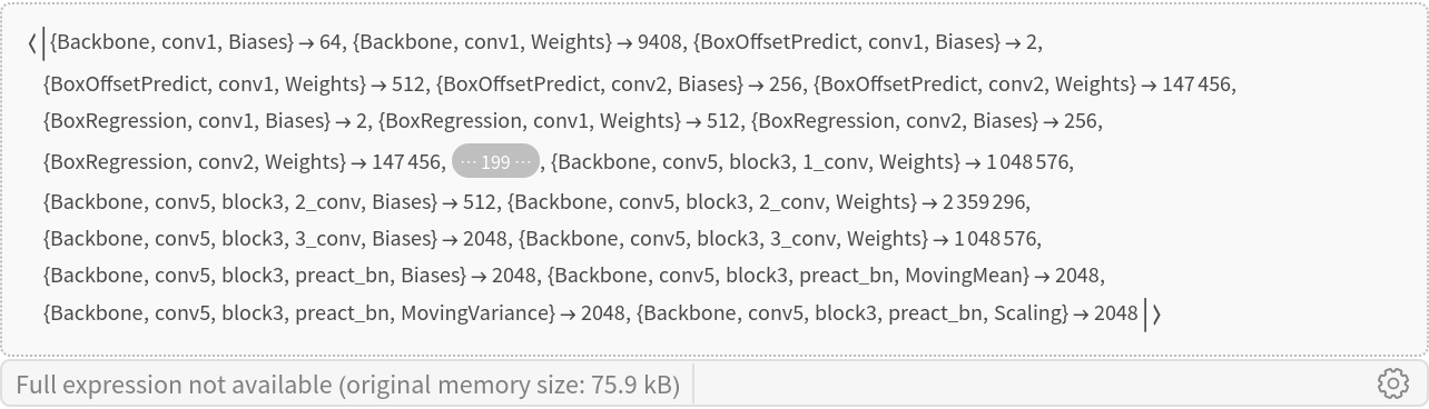
Inspect the number of parameters of all arrays in the net:
Obtain the total number of parameters:
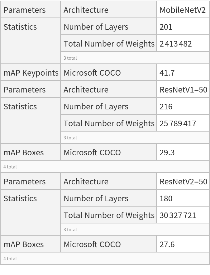
Obtain the layer type counts:
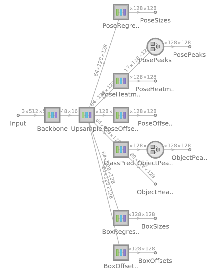
Display the summary graphic:
![(* Evaluate this cell to get the example input *) CloudGet["https://www.wolframcloud.com/obj/96ac21ef-3eb3-460b-8ae9-31fa3977a291"]](https://www.wolframcloud.com/obj/resourcesystem/images/ad9/ad9e7395-15c4-4423-b9b5-f3f82e31be30/0e09cac1643eb1a2.png)
![Options[netevaluate] = Join[Options[alignKeypoints], Options[decode]];
netevaluate[net_, img_Image, opts : OptionsPattern[]] := Block[
{scale, predictions},
predictions = decode[net, img, Sequence @@ DeleteCases[{opts}, "NeighborhoodRadius" | "FilterOutsideDetections" -> _]];
scale = Max@N[ImageDimensions[img]/
Reverse@Rest@NetExtract[net, NetPort["PosePeaks"]]]; alignKeypoints[predictions,
"FilterOutsideDetections" -> OptionValue["FilterOutsideDetections"],
"NeighborhoodRadius" -> OptionValue["NeighborhoodRadius"]*scale
]
]](https://www.wolframcloud.com/obj/resourcesystem/images/ad9/ad9e7395-15c4-4423-b9b5-f3f82e31be30/3b2bf07f18b36d46.png)
![(* Evaluate this cell to get the example input *) CloudGet["https://www.wolframcloud.com/obj/1ac8b227-06bb-4acf-bf64-123358367291"]](https://www.wolframcloud.com/obj/resourcesystem/images/ad9/ad9e7395-15c4-4423-b9b5-f3f82e31be30/521fe7842223f455.png)

![{{1, 2}, {1, 3}, {2, 4}, {3, 5}, {1, 6}, {1, 7}, {6, 8}, {8, 10}, {7, 9}, {9, 11}, {6, 7}, {6, 12}, {7, 13}, {12, 13}, {12, 14}, {14, 16}, {13, 15}, {15, 17}};
getSkeleton[personKeypoints_] := Line[DeleteMissing[
Map[personKeypoints[[#]] &, {{1, 2}, {1, 3}, {2, 4}, {3, 5}, {1, 6}, {1, 7}, {6, 8}, {8, 10}, {7, 9}, {9, 11}, {6, 7}, {6, 12}, {7,
13}, {12, 13}, {12, 14}, {14, 16}, {13, 15}, {15, 17}}], 1, 2]]](https://www.wolframcloud.com/obj/resourcesystem/images/ad9/ad9e7395-15c4-4423-b9b5-f3f82e31be30/320fc4e7eac8a0b0.png)
![HighlightImage[testImage,
Append[
AssociationThread[Range[Length[#]] -> #] & /@ {keypoints, Map[getSkeleton, keypoints]},
GroupBy[predictions["ObjectDetection"][[All, ;; 2]], Last -> First]
],
ImageLabels -> None
]](https://www.wolframcloud.com/obj/resourcesystem/images/ad9/ad9e7395-15c4-4423-b9b5-f3f82e31be30/001d523a220a2f9f.png)
![(* Evaluate this cell to get the example input *) CloudGet["https://www.wolframcloud.com/obj/2e67ed23-827d-4440-a269-cb17a44084bb"]](https://www.wolframcloud.com/obj/resourcesystem/images/ad9/ad9e7395-15c4-4423-b9b5-f3f82e31be30/7d2c155ffaa3464d.png)
![predictions = netevaluate[
NetModel["CenterNet Pose Estimation Nets Trained on MS-COCO Data"],
testImage2, "ObjectDetectionThreshold" -> 0.28, "HumanPoseThreshold" -> 0.2, "FilterOutsideDetections" -> True];
keypoints = predictions["KeypointEstimation"];](https://www.wolframcloud.com/obj/resourcesystem/images/ad9/ad9e7395-15c4-4423-b9b5-f3f82e31be30/4e43bd0047bce481.png)
![HighlightImage[testImage2,
AssociationThread[Range[Length[#]] -> #] & /@ {keypoints, Map[getSkeleton, keypoints], predictions[["ObjectDetection", All, 1]]}
, ImageLabels -> None]](https://www.wolframcloud.com/obj/resourcesystem/images/ad9/ad9e7395-15c4-4423-b9b5-f3f82e31be30/254183d511f3d625.png)
![Grid@List@Table[
predictions = netevaluate[
NetModel[
"CenterNet Pose Estimation Nets Trained on MS-COCO Data"], testImage2, "ObjectDetectionThreshold" -> 0.28, "HumanPoseThreshold" -> 0.2, "NeighborhoodRadius" -> r,
"FilterOutsideDetections" -> False
];
HighlightImage[testImage2,
AssociationThread[Range[Length[#]] -> #] & /@ {predictions[
"KeypointEstimation"], Map[getSkeleton, predictions["KeypointEstimation"]], predictions[["ObjectDetection", All, 1]]}
, ImageLabels -> None],
{r, {1, 5, 8}}
]](https://www.wolframcloud.com/obj/resourcesystem/images/ad9/ad9e7395-15c4-4423-b9b5-f3f82e31be30/26699bb056324d40.png)

![res = Map[Transpose[#, {3, 2, 1}] &, res];
res["BoxOffsets"] = Map[Reverse, res["BoxOffsets"], {2}];
res["BoxSizes"] = Map[Reverse, res["BoxSizes"], {2}];](https://www.wolframcloud.com/obj/resourcesystem/images/ad9/ad9e7395-15c4-4423-b9b5-f3f82e31be30/3a1091618fb987c6.png)

![Graphics[
MapThread[{EdgeForm[Opacity[Total[#1]*0.5]], #2} &, {Flatten@
Map[Max, res["ObjectHeatmaps"], {2}], Map[boxDecoder[#, {128, 128}, 1] &, boxes]}],
BaseStyle -> {FaceForm[], EdgeForm[{Thin, Black}]}
]](https://www.wolframcloud.com/obj/resourcesystem/images/ad9/ad9e7395-15c4-4423-b9b5-f3f82e31be30/23619b17e8a0a9c6.png)

![Graphics[
MapThread[{EdgeForm[Opacity[#1]], Rectangle @@ #2} &, {Flatten[
res["ObjectHeatmaps"][[All, All, idx]]], Map[boxDecoder[#, {128, 128}, 1] &, boxes]}],
BaseStyle -> {FaceForm[], EdgeForm[{Thin, Black}]}
]](https://www.wolframcloud.com/obj/resourcesystem/images/ad9/ad9e7395-15c4-4423-b9b5-f3f82e31be30/119605e938c34212.png)

![HighlightImage[testImage, Graphics[
MapThread[{EdgeForm[{Opacity[#1]}], #2} &, {Flatten[
res["ObjectHeatmaps"][[All, All, idx]]], Map[boxDecoder[#, ImageDimensions[testImage], Max@N[ImageDimensions[testImage]/{128, 128}]] &, boxes]}]], BaseStyle -> {FaceForm[], EdgeForm[{Thin, Red}]}]](https://www.wolframcloud.com/obj/resourcesystem/images/ad9/ad9e7395-15c4-4423-b9b5-f3f82e31be30/69fc75d7f1444716.png)
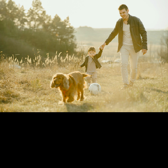
![(* Evaluate this cell to get the example input *) CloudGet["https://www.wolframcloud.com/obj/cb65e6fb-7b1b-49ea-af60-8df89bc2ec56"]](https://www.wolframcloud.com/obj/resourcesystem/images/ad9/ad9e7395-15c4-4423-b9b5-f3f82e31be30/58795eb06da65349.png)
![objectHeatmaps = NetModel["CenterNet Pose Estimation Nets Trained on MS-COCO Data"][
testImage]["ObjectHeatmaps"];](https://www.wolframcloud.com/obj/resourcesystem/images/ad9/ad9e7395-15c4-4423-b9b5-f3f82e31be30/7d8db2e6cdd676db.png)
![idx = Position[labels, "dog"][[1, 1]];
strengthArray = objectHeatmaps[[idx]];
heatmap = ImageApply[{#, 1 - #, 1 - #} &, ImageAdjust@Image[strengthArray]];
heatmap = ImageTake[
ImageResize[heatmap, {Max[#]}], {1, Last[#]}, {1, First[#]}] &@
ImageDimensions[testImage]](https://www.wolframcloud.com/obj/resourcesystem/images/ad9/ad9e7395-15c4-4423-b9b5-f3f82e31be30/321ac81e97038bb0.png)
![visualizeHeatmap[img_Image, heatmap_] := Block[{strengthArray, w, h},
{w, h} = ImageDimensions[img];
strengthArray = Map[Max, Transpose[heatmap, {3, 1, 2}], {2}];
strengthArray = ImageApply[{#, 1 - #, 1 - #} &, ImageAdjust@Image[strengthArray]];
strengthArray = ImageTake[ImageResize[strengthArray, {Max[w, h]}], {1, h}, {1, w}];
ImageCompose[img, {ColorConvert[strengthArray, "RGB"], 0.4}]
];](https://www.wolframcloud.com/obj/resourcesystem/images/ad9/ad9e7395-15c4-4423-b9b5-f3f82e31be30/3d38b07500ce612a.png)
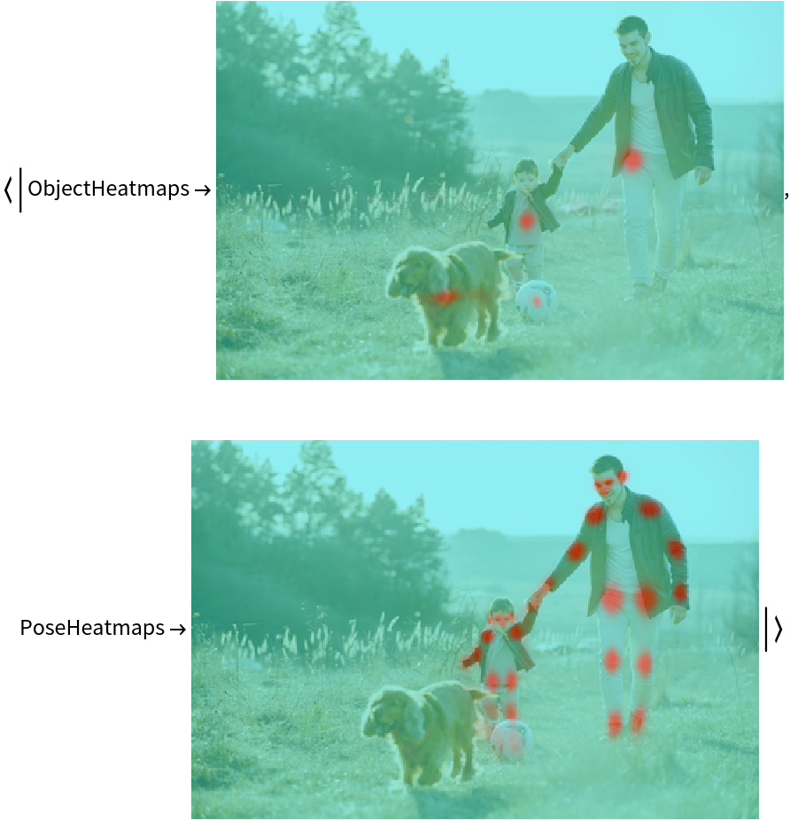
![Map[visualizeHeatmap[testImage, #] &, NetModel["CenterNet Pose Estimation Nets Trained on MS-COCO Data"][
testImage, {"ObjectHeatmaps", "PoseHeatmaps"}]]](https://www.wolframcloud.com/obj/resourcesystem/images/ad9/ad9e7395-15c4-4423-b9b5-f3f82e31be30/699b75b4dd08ae90.png)
![newEncoder = NetEncoder[{"Image", {320, 320}, Method -> "Fit", Alignment -> {Left, Top}, "MeanImage" -> NetExtract[encoder, "MeanImage"], "VarianceImage" -> NetExtract[encoder, "VarianceImage"]}]](https://www.wolframcloud.com/obj/resourcesystem/images/ad9/ad9e7395-15c4-4423-b9b5-f3f82e31be30/50fd580537e9aa9d.png)
![resizedNet = NetReplacePart[
NetModel["CenterNet Pose Estimation Nets Trained on MS-COCO Data"], "Input" -> newEncoder]](https://www.wolframcloud.com/obj/resourcesystem/images/ad9/ad9e7395-15c4-4423-b9b5-f3f82e31be30/2024829dd5a45d33.png)