Resource retrieval
Get the pre-trained net:
NetModel parameters
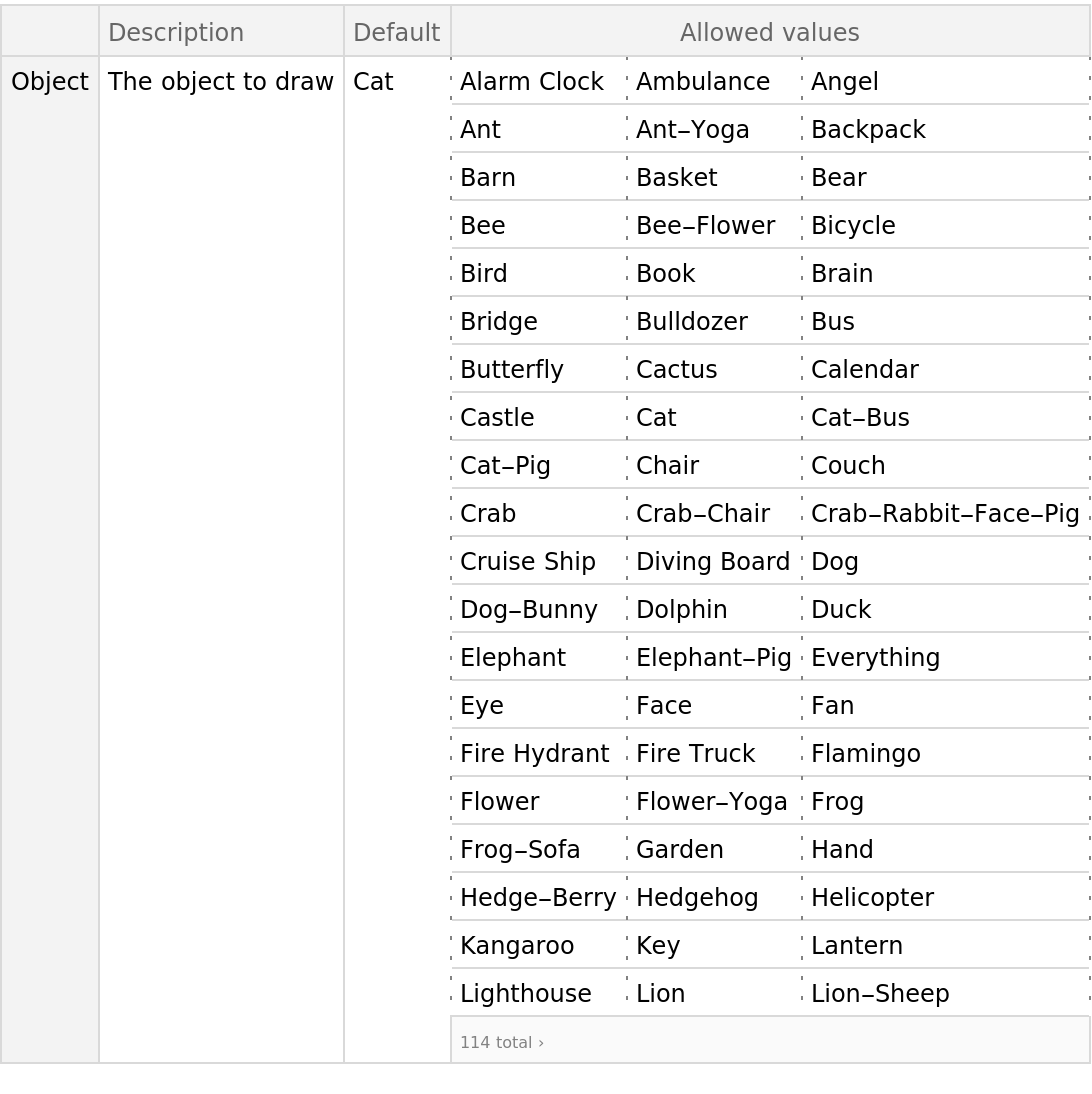
This model consists of a family of individual nets, each identified by a specific parameter combination. Inspect the available parameters and their default values:
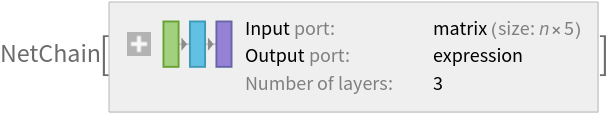
Pick a non-default net by specifying the parameters:
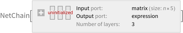
Pick a non-default uninitialized net:
Check the default parameter combination:
Evaluation function
Define an evaluation function to generate a sketch from a fixed initial condition using temperature sampling:
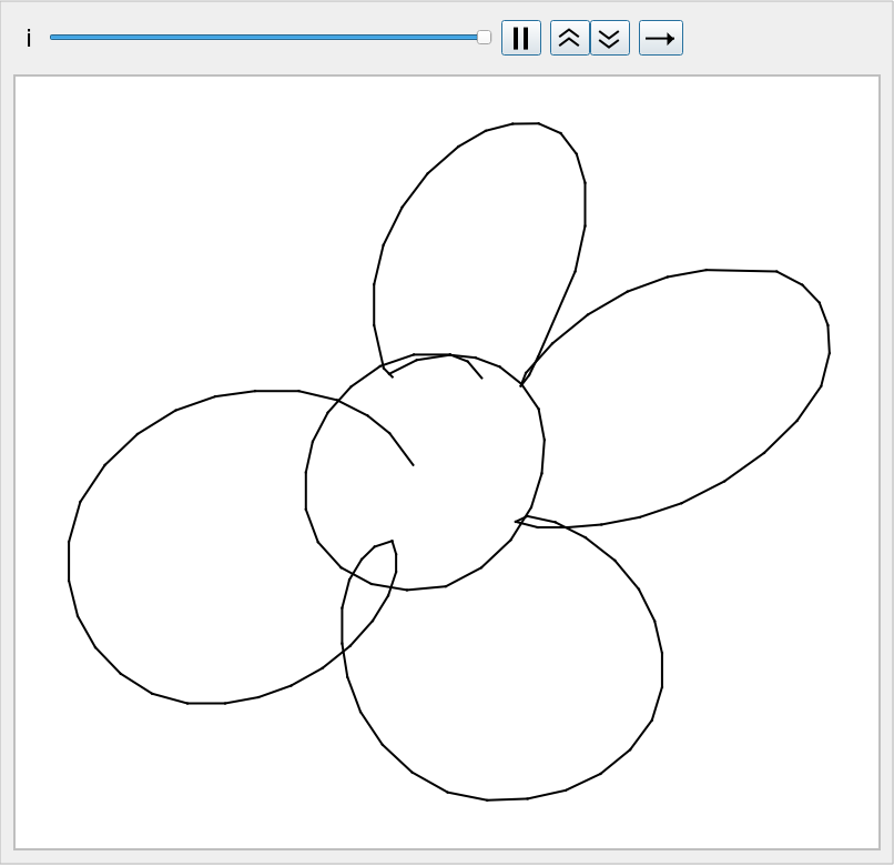
Basic usage
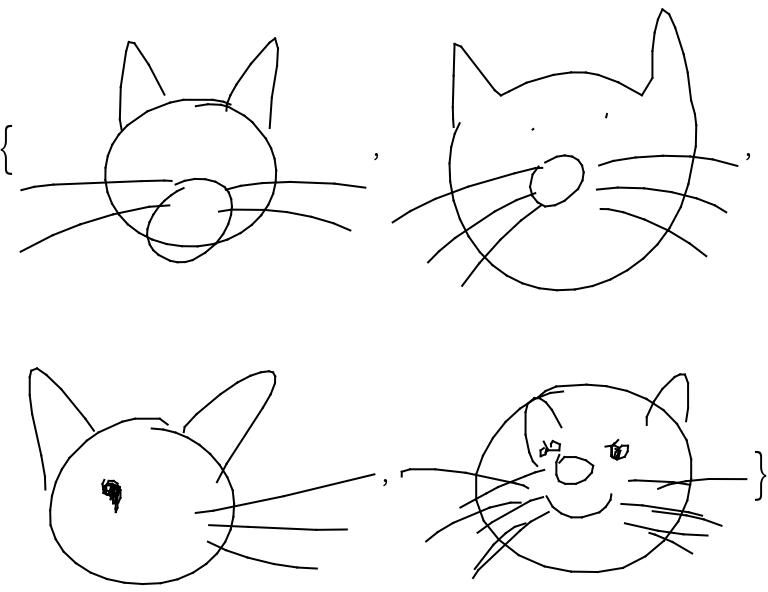
Generate four sketches of a cat:
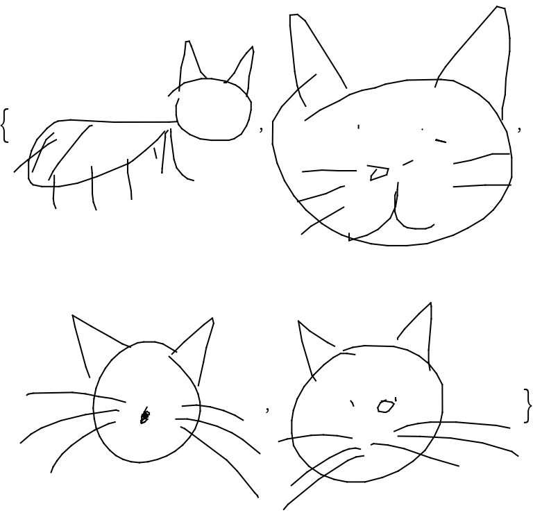
The third optional argument is a “temperature” parameter that regulates sampling. A higher temperature increases the variability in the output, increasing the probability of sampling less likely strokes:
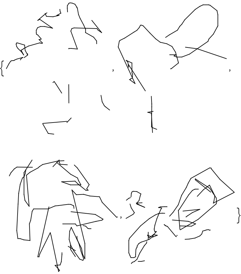
Very high temperature settings are equivalent to sampling from a flat distribution:
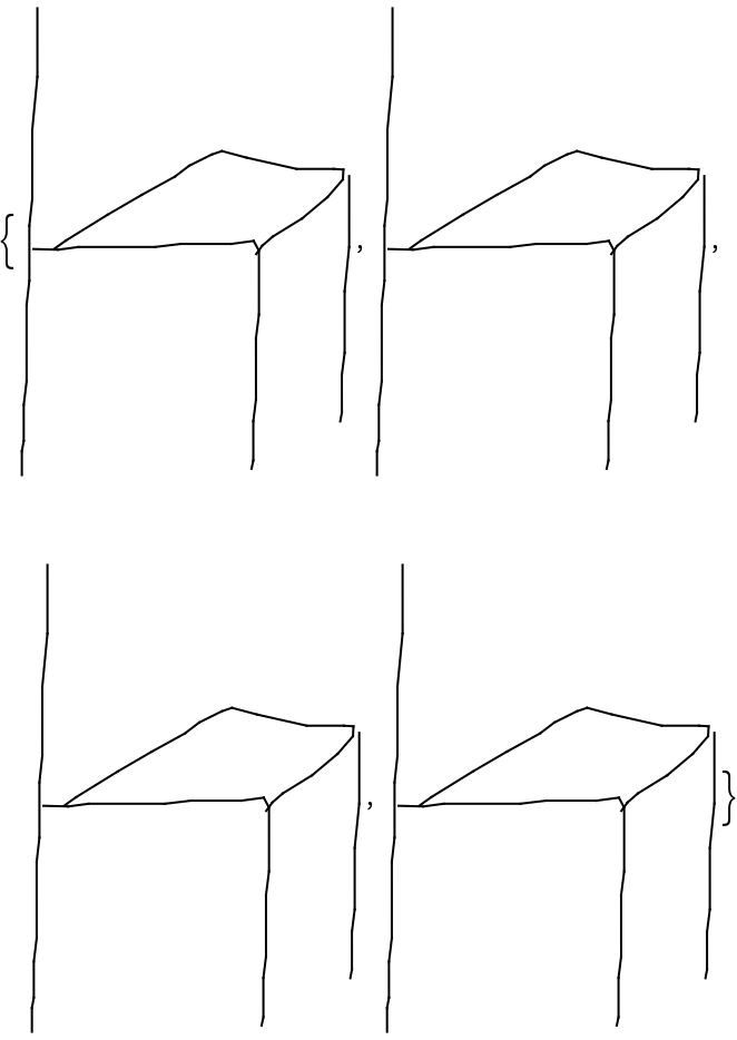
Very low temperature settings further increase the probability of extracting more likely strokes. Sampling at zero temperature is equivalent to always picking the stroke with maximum probability, and the function produces the same sketch every time:
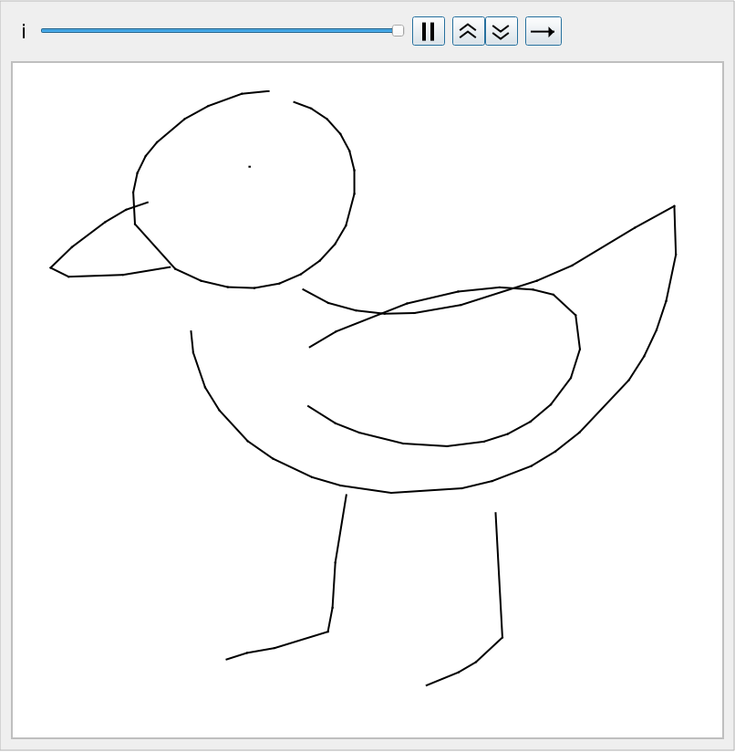
Visualize the sequence of pen strokes
Create a function which displays an animation showing the object being drawn from the sequence of pen strokes chosen by the network:
Sketch representation
This model represents sketches as a sequence of pen strokes, each identified as a vector of five elements: {Δx, Δy, p1, p2, p3}. The elements {Δx, Δy} represent the pen movement in the sketch plane, while {p1, p2, p3} is a one-hot vector representing the state of the pen. The state {1, 0, 0} indicates that the pen is touching the paper and a segment will be drawn, {0, 1, 0} means the pen is not touching the paper and {0, 0, 1} indicates that the sketch is finished:
The model works like a language model, reading a sequence of pen strokes and predicting the next one:
Decoder properties
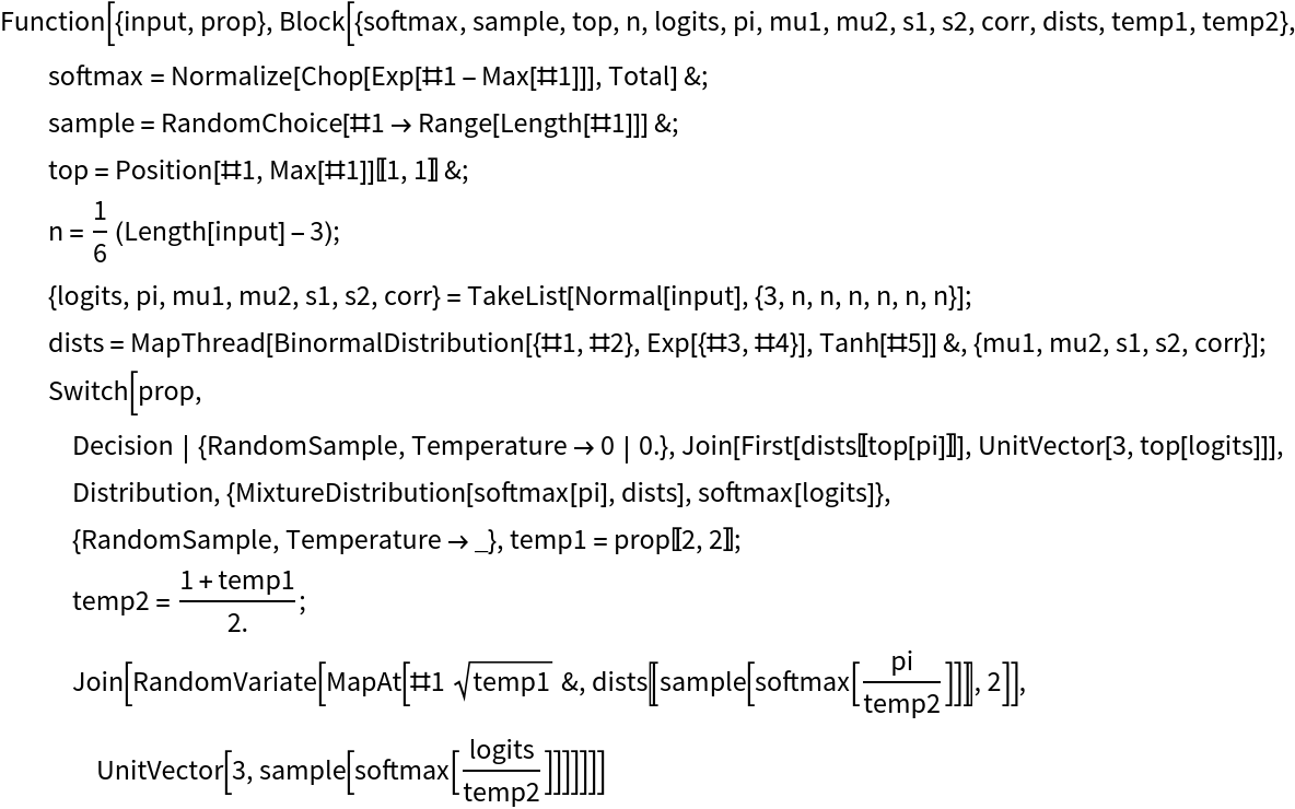
Extract the “Function” net decoder:
Inspect the associated Function:
This decoder supports properties. The default one, “Decision”, returns the pen stroke with highest associated probability:
It is possible to perform temperature sampling from the output distribution with the property “RandomSample”. In this case, the evaluation will return different results every time:
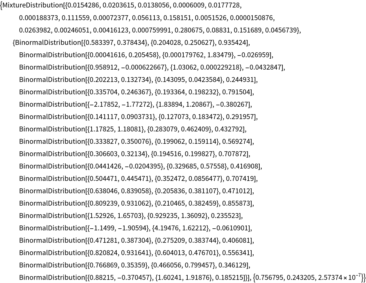
The property “Distribution” returns the full probability distribution for the stroke direction and the pen state. The stroke direction distribution is a mixture of two-dimensional normal distributions, while the distribution of the pen state is a categorical distribution with three probability values for 1, 2 and 3:
Net information
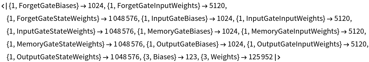
Inspect the number of parameters of all arrays in the net:
Obtain the total number of parameters:
Obtain the layer type counts:
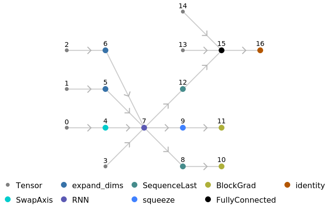
Display the summary graphic:
Export to MXNet
Export the net into a format that can be opened in MXNet:
Export also creates a net.params file containing parameters:
Get the size of the parameter file:
Represent the MXNet net as a graph:
![drawSketch[obj_, temp_ : 0.01, maxLen_ : 300] := Block[{stateObject, lastPos, pos, stroke, segments, time, lastAction, action, offset}, stateObject = NetStateObject@
NetModel[{"Sketch-RNN Trained on QuickDraw Data", "Object" -> obj}];
lastPos = pos = {0, 0};
stroke = {0, 0, 0, 0, 0};
segments = Table[{}, maxLen];
time = 0; action = 1;
While[time++ < maxLen,
lastAction = action;
stroke = stateObject[{stroke}, {"RandomSample", "Temperature" -> N@temp}];
offset = stroke[[;; 2]];
action = First@Ordering[stroke[[3 ;;]], -1];
lastPos = pos;
pos += offset*{1, -1};
Switch[lastAction,
1, segments[[time]] = {lastPos, pos},
3, Break[]]
];
segments
];](https://www.wolframcloud.com/obj/resourcesystem/images/373/3733fed3-f297-454c-b18e-3789ac74856c/185980e1dca6b691.png)
![animateSketch[obj_] := DynamicModule[{lines, plotRange},
lines = DeleteCases[drawSketch[obj], {}];
plotRange = Map[MinMax, 1.05*{lines[[All, All, 1]], lines[[All, All, 2]]}];
Animate[
Graphics[Line@lines[[1 ;; i]], PlotRange -> plotRange],
{i, 1, Length[lines], 1},
AnimationRepetitions -> 1
]
]](https://www.wolframcloud.com/obj/resourcesystem/images/373/3733fed3-f297-454c-b18e-3789ac74856c/36bda8cba3304f90.png)


![jsonPath = Export[FileNameJoin[{$TemporaryDirectory, "net.json"}], NetReplacePart[NetModel["Sketch-RNN Trained on QuickDraw Data"], "Input" -> {50, 5}], "MXNet"]](https://www.wolframcloud.com/obj/resourcesystem/images/373/3733fed3-f297-454c-b18e-3789ac74856c/36f042df73f8875b.png)