Resource retrieval
Get the pre-trained net:
NetModel parameters
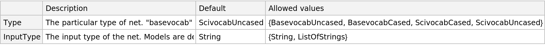
This model consists of a family of individual nets, each identified by a specific parameter combination. Inspect the available parameters:
Pick a non-default net by specifying the parameters:
Pick a non-default uninitialized net:
Basic usage
Given a piece of text, SciBERT net produces a sequence of feature vectors of size 768, which corresponds to the sequence of input words or subwords:
Obtain the dimensions of the embeddings:
Visualize the embeddings:
Transformer architecture
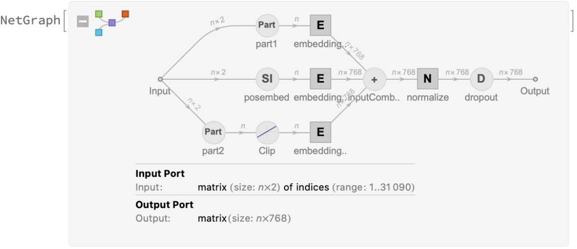
Each input text segment is first tokenized into words or subwords using a word-piece tokenizer and additional text normalization. Integer codes called token indices are generated from these tokens, together with additional segment indices:
For each input subword token, the encoder yields a pair of indices that corresponds to the token index in the vocabulary and the index of the sentence within the list of input sentences:
The list of tokens always starts with special token index 102, which corresponds to the classification index.
Also the special token index 103 is used as a separator between the different text segments. Each subword token is also assigned a positional index:
A lookup is done to map these indices to numeric vectors of size 768:
For each subword token, these three embeddings are combined by summing elements with ThreadingLayer:
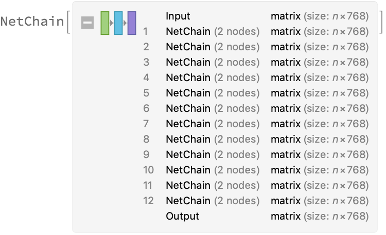
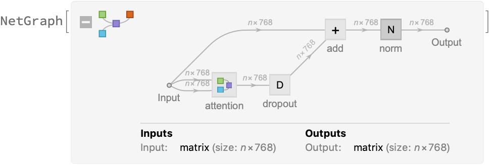
The transformer architecture then processes the vectors using 12 structurally identical self-attention blocks stacked in a chain:
The key part of these blocks is the attention module comprising of 12 parallel self-attention transformations, also called “attention heads.” Each head uses an AttentionLayer at its core:
SciBERT uses self-attention, where the embedding of a given subword depends on the full input text. The following figure compares self-attention (lower left) to other types of connectivity patterns that are popular in deep learning:
Sentence analogies
Define a sentence embedding that takes the last feature vector from SciBERT subword embeddings (as an arbitrary choice):
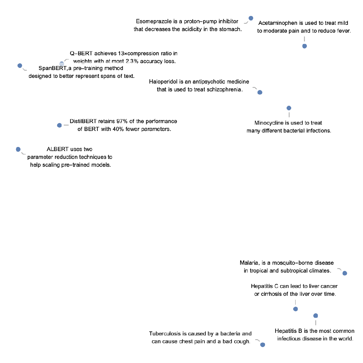
Define a list of sentences in three broad categories (diseases, medicines and NLP models):
Precompute the embeddings for a list of sentences:
Visualize the similarity between the sentences using the net as a feature extractor:
Net information
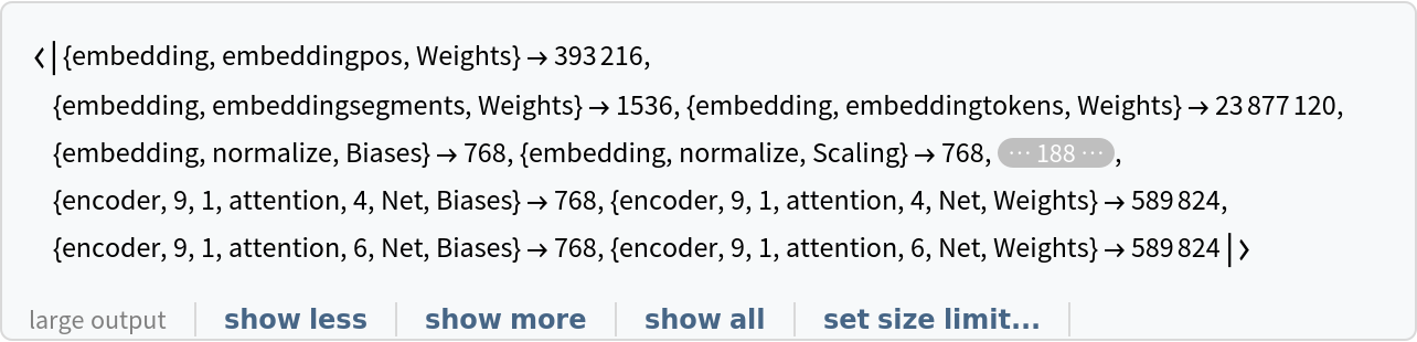
Inspect the number of parameters of all arrays in the net:
Obtain the total number of parameters:
Obtain the layer type counts:
Display the summary graphic:
Export to MXNet
Export the net into a format that can be opened in MXNet:
Export also creates a net.params file containing parameters:
Get the size of the parameter file:
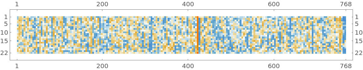
![input = "Cushing syndrome symptoms with adrenal suppression is caused by a exogenous glucocorticoid depot triamcinolone.";
embeddings = NetModel["SciBERT Trained on Semantic Scholar Data"][input];](https://www.wolframcloud.com/obj/resourcesystem/images/ae4/ae4e599e-1e68-4fef-ba6a-777012f5a4e0/0e9209c5336bfc59.png)

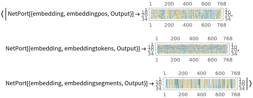
![net[{"The patient was on clindamycin and topical tazarotene for his acne.", "His family history included hypertension, diabetes, and heart disease."}, NetPort[{"embedding", "posembed", "Output"}]]](https://www.wolframcloud.com/obj/resourcesystem/images/ae4/ae4e599e-1e68-4fef-ba6a-777012f5a4e0/0db80d0194575c68.png)
![embeddings = net[{"The patient was on clindamycin and topical tazarotene for his acne.", "His family history included hypertension, diabetes, and heart disease."},
{NetPort[{"embedding", "embeddingpos", "Output"}],
NetPort[{"embedding", "embeddingtokens", "Output"}],
NetPort[{"embedding", "embeddingsegments", "Output"}]}];
Map[MatrixPlot, embeddings]](https://www.wolframcloud.com/obj/resourcesystem/images/ae4/ae4e599e-1e68-4fef-ba6a-777012f5a4e0/4d4333efb0a31d1d.png)
![sentences = {"Hepatitis B is the most common infectious disease in the world.", "Malaria, is a mosquito-borne disease in tropical and subtropical climates.", "Hepatitis C can lead to liver cancer or cirrhosis of the liver over time.", "Tuberculosis is caused by a bacteria and can cause chest pain and a bad cough.",
"Acetaminophen is used to treat mild to moderate pain and to reduce fever.",
"Esomeprazole is a proton-pump inhibitor that decreases the acidicity in the stomach.",
"Haloperidol is an antipsychotic medicine that is used to treat schizophrenia.",
"Minocycline is used to treat many different bacterial infections.",
"SpanBERT,a pre-training method designed to better represent spans of text.", "ALBERT uses two parameter reduction techniques to help scaling pre-trained models.",
"DistilBERT retains 97% of the performance of BERT with 40% fewer parameters.",
"Q-BERT achieves 13\[Times]compression ratio in weights with at most 2.3% accuracy loss."};](https://www.wolframcloud.com/obj/resourcesystem/images/ae4/ae4e599e-1e68-4fef-ba6a-777012f5a4e0/3ee32b6f7522924d.png)