ResNet-101
Trained on
YFCC100m Geotagged Data
Released in 2017, this geolocation model classifies the location in which a photo was taken among more than 15,000 predefined locations around the world. The classes correspond to cells extracted from Google's S2 Geometry library.
Number of layers: 344 |
Parameter count: 74,405,235 |
Trained size: 299 MB |
Examples
Resource retrieval
Get the pre-trained net:
Basic Usage
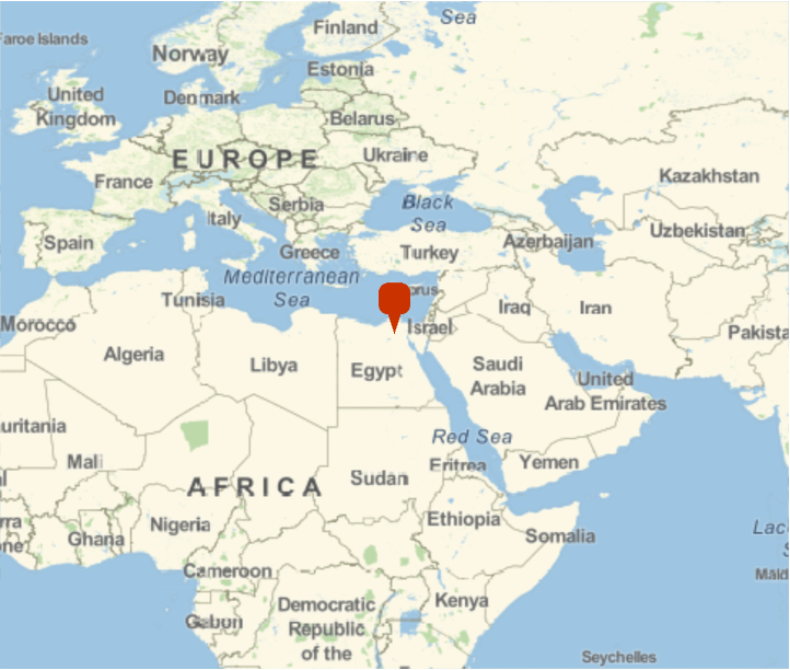
Obtain an estimate of the latitude and longitude of where a photo was taken:
Show a map of the area corresponding to the position:
Mark the position on a world map:
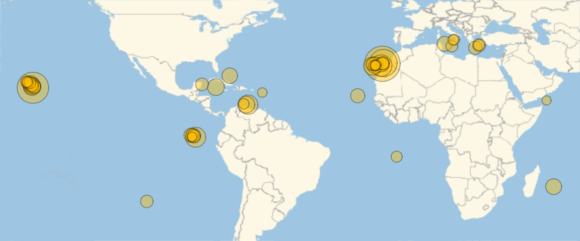
Multiple Predictions
The net returns a probability distribution over all available locations. Obtain the 50 most probable locations for a given image and plot these locations on the world map, with the size of the location marker proportional to the probability:
Fine Scale Predictions
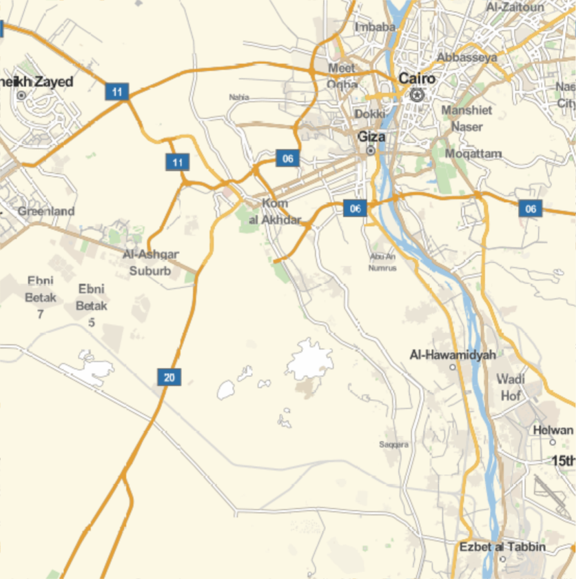
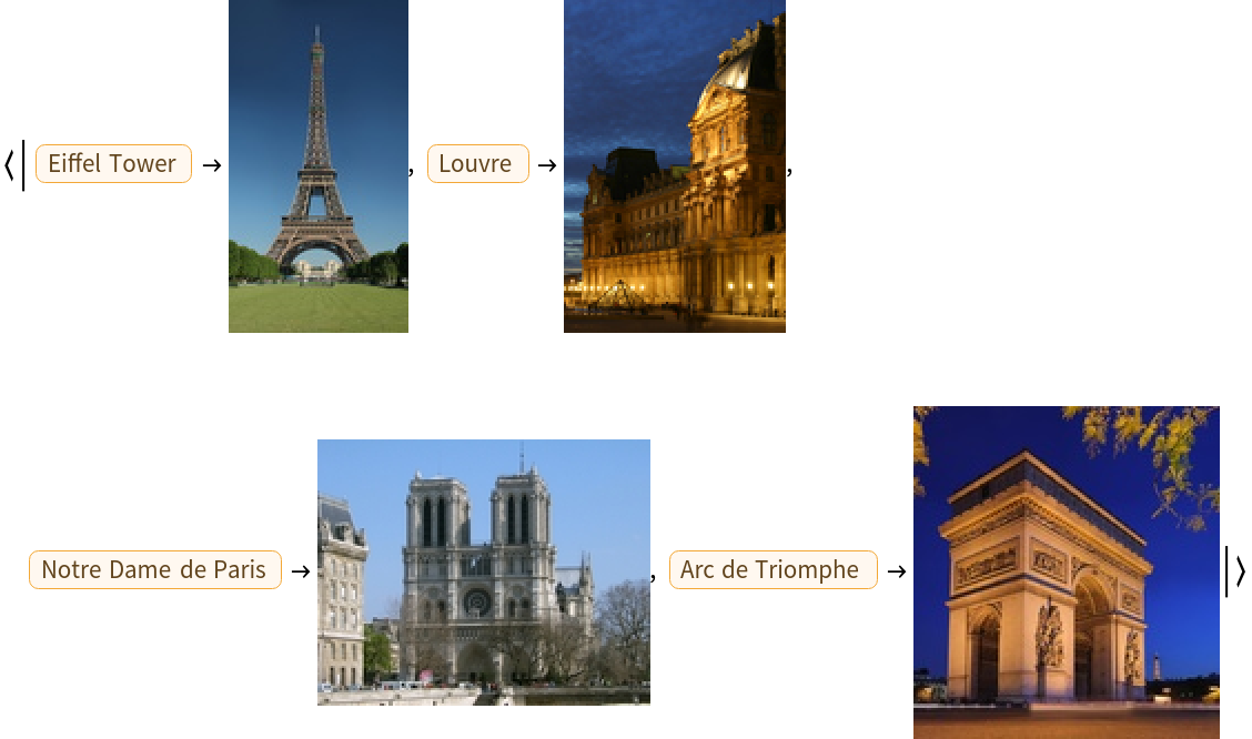
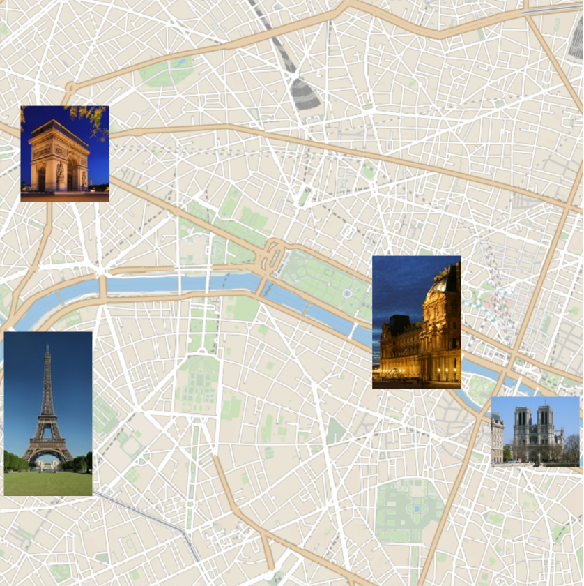
In places with high population density, very fine-grained predictions are possible. Consider the following four landmarks in Paris:
Predict the locations of the four landmarks and mark the locations on the map:
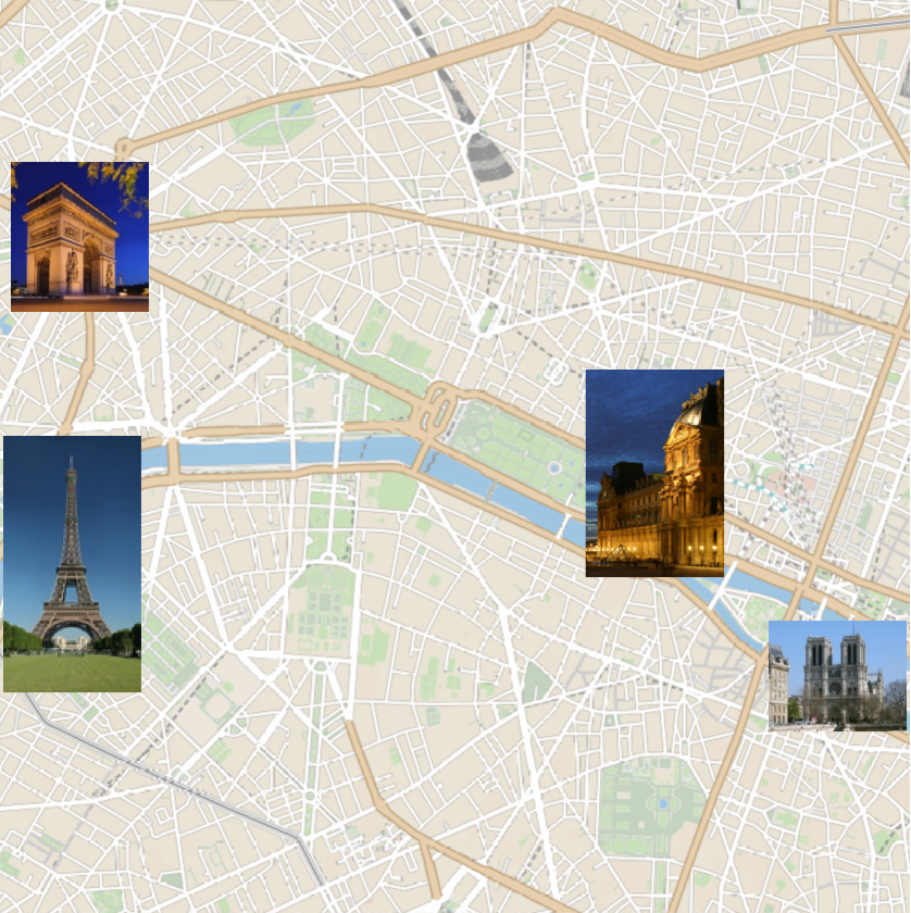
Compare with the actual locations:
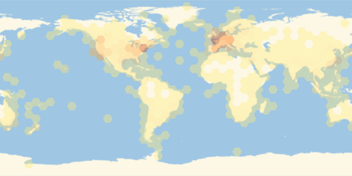
Region Density
Inspect the distribution of the available positions. Display a heat map of the location density on the map:
Net information
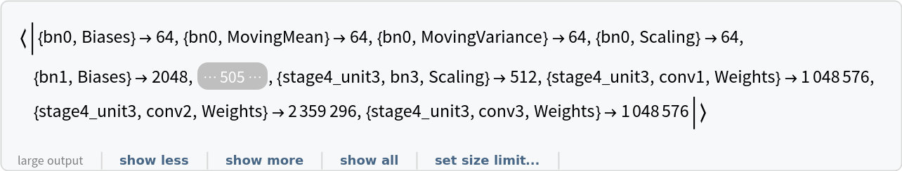
Inspect the number of parameters of all arrays in the net:
Obtain the total number of parameters:
Obtain the layer type counts:
Display the summary graphic:
Export to MXNet
Export the net into a format that can be opened in MXNet:
Export also creates a net.params file containing parameters:
Get the size of the parameter file:
The size is similar to the byte count of the resource object:
Requirements
Wolfram Language
11.2
(September 2017)
or above
External Links
Resource History
Reference
![(* Evaluate this cell to get the example input *) CloudGet["https://www.wolframcloud.com/obj/05b39d48-9143-493f-a90e-bc264abf15f0"]](https://www.wolframcloud.com/obj/resourcesystem/images/26c/26c74bb9-4e37-4b95-95f0-accfd294901d/6997d64e0196aa28.png)
![(* Evaluate this cell to get the example input *) CloudGet["https://www.wolframcloud.com/obj/77685f62-27fe-4ce8-8a10-46032783db50"]](https://www.wolframcloud.com/obj/resourcesystem/images/26c/26c74bb9-4e37-4b95-95f0-accfd294901d/5d3a95372bce22fe.png)
![landmarks = EntityValue[{Entity["Building", "EiffelTower::5h9w8"], Entity["Building", "TheLouvre::vqy3g"], Entity["Building", "NotreDameCathedral::95fcw"], Entity["Building", "ArcDeTriomphe::92x88"]}, "Image", "EntityAssociation"]](https://www.wolframcloud.com/obj/resourcesystem/images/26c/26c74bb9-4e37-4b95-95f0-accfd294901d/7556fdff674cf0b5.png)
![GeoListPlot[
MapThread[
GeoMarker[#1, #2, "Scale" -> 0.01] &, {NetModel[
"ResNet-101 Trained on YFCC100m Geotagged Data"][
Values[landmarks]], Values[landmarks]}], GeoRange -> Quantity[1.5, "Miles"]]](https://www.wolframcloud.com/obj/resourcesystem/images/26c/26c74bb9-4e37-4b95-95f0-accfd294901d/56cbf357e855c1b5.png)
![GeoListPlot[
Map[GeoMarker[EntityValue[#, "Position"], EntityValue[#, "Image"], "Scale" -> 0.01] &, Keys[landmarks]], GeoRange -> Quantity[1.5, "Miles"]]](https://www.wolframcloud.com/obj/resourcesystem/images/26c/26c74bb9-4e37-4b95-95f0-accfd294901d/2da896eb25ea1dcf.png)
![GeoHistogram[
NetExtract[NetModel["ResNet-101 Trained on YFCC100m Geotagged Data"],
"Output"][["Labels"]], 50, PlotStyle -> Opacity[0.4], ImageSize -> Large]](https://www.wolframcloud.com/obj/resourcesystem/images/26c/26c74bb9-4e37-4b95-95f0-accfd294901d/29137f8173e293ad.png)
![NetInformation[
NetModel[
"ResNet-101 Trained on YFCC100m Geotagged Data"], "ArraysElementCounts"]](https://www.wolframcloud.com/obj/resourcesystem/images/26c/26c74bb9-4e37-4b95-95f0-accfd294901d/141ff914dcf5da46.png)
![NetInformation[
NetModel[
"ResNet-101 Trained on YFCC100m Geotagged Data"], "ArraysTotalElementCount"]](https://www.wolframcloud.com/obj/resourcesystem/images/26c/26c74bb9-4e37-4b95-95f0-accfd294901d/0e48dbaab649c406.png)
![NetInformation[
NetModel[
"ResNet-101 Trained on YFCC100m Geotagged Data"], "LayerTypeCounts"]](https://www.wolframcloud.com/obj/resourcesystem/images/26c/26c74bb9-4e37-4b95-95f0-accfd294901d/16a218b0c8a1555f.png)
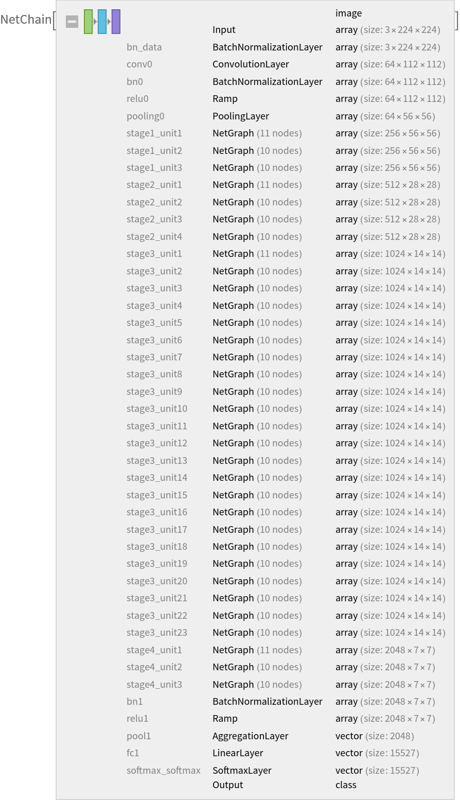
![NetInformation[
NetModel[
"ResNet-101 Trained on YFCC100m Geotagged Data"], "SummaryGraphic"]](https://www.wolframcloud.com/obj/resourcesystem/images/26c/26c74bb9-4e37-4b95-95f0-accfd294901d/12201015020e0d34.png)
![jsonPath = Export[FileNameJoin[{$TemporaryDirectory, "net.json"}], NetModel["ResNet-101 Trained on YFCC100m Geotagged Data"], "MXNet"]](https://www.wolframcloud.com/obj/resourcesystem/images/26c/26c74bb9-4e37-4b95-95f0-accfd294901d/2bbcafcfd91ab84a.png)