Resource retrieval
Get the pre-trained net:
NetModel parameters
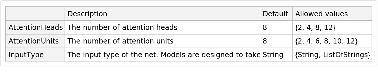
This model consists of a family of individual nets, each identified by a specific parameter combination. Inspect the available parameters:
Pick a non-default net by specifying the parameters:
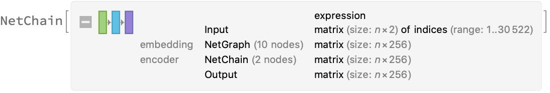
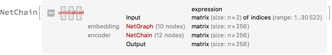
Pick a non-default uninitialized net:
Basic usage
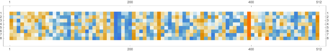
Given a piece of text, the default pre-trained distilled BERT net produces a sequence of feature vectors of size 512 (in general, the size of the feature vector is 64 × "AttentionHeads"), which corresponds to the sequence of input words or subwords:
Obtain dimensions of the embeddings:
Visualize the embeddings:
Transformer architecture
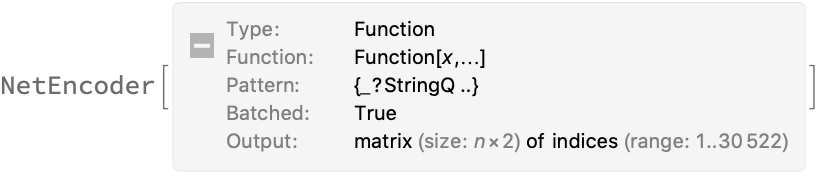
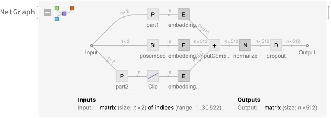
Each input text segment is first tokenized into words or subwords using a word-piece tokenizer and additional text normalization. Integer codes called token indices are generated from these tokens, together with additional segment indices:
For each input subword token, the encoder yields a pair of indices that corresponds to the token index in the vocabulary and the index of the sentence within the list of input sentences:
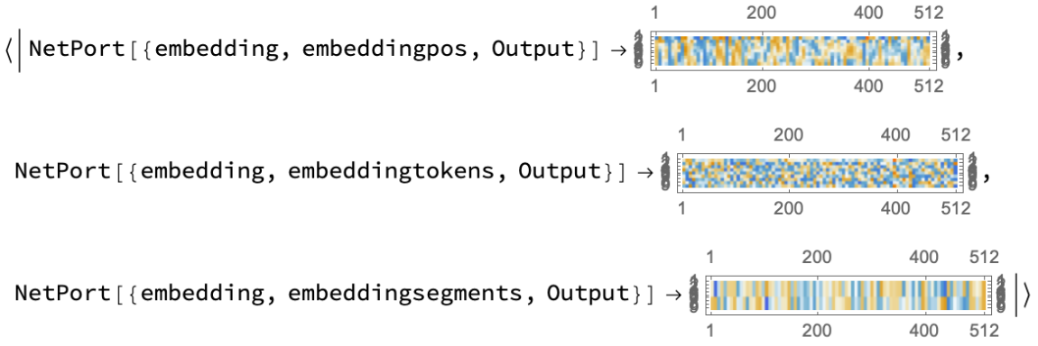
The list of tokens always starts with special token index 102, which corresponds to the classification index.
Also, the special token index 103 is used as a separator between the different text segments. Each subword token is also assigned a positional index:
A lookup is done to map these indices to numeric vectors of size 512:
For each subword token, these three embeddings are combined by summing elements with ThreadingLayer:
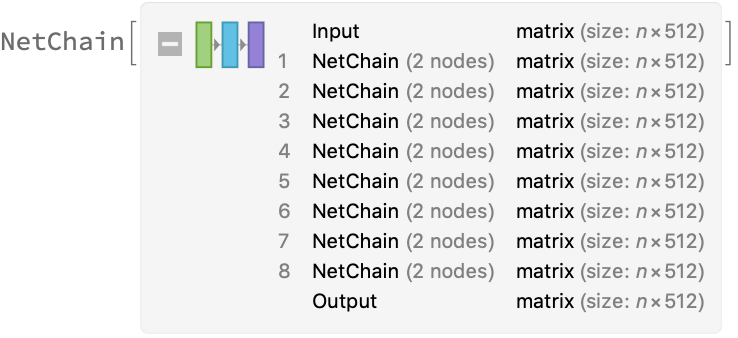
The transformer architecture then processes the vectors using six structurally identical self-attention blocks stacked in a chain:
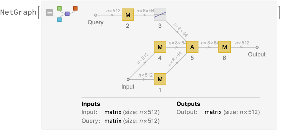
The key part of these blocks is the attention module comprising of parallel self-attention transformations, also called "AttentionHeads". The number of such blocks is given by the parameter "AttentionUnits":
BERT-like models use self-attention, where the embedding of a given subword depends on the full input text. The following figure compares self-attention (lower left) to other types of connectivity patterns that are popular in deep learning:
Sentence analogies
Define a sentence embedding that takes the last feature vector from pre-trained distilled BERT subword embeddings (as an arbitrary choice):
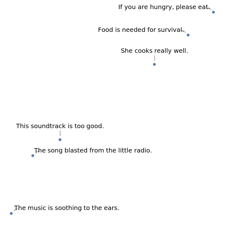
Define a list of sentences:
Precompute the embeddings for a list of sentences:
Visualize the similarity between the sentences using the net as a feature extractor:
Train a classifier model with the subword embeddings
Get a text-processing dataset:
View a random sample of the dataset:
Precompute the pre-trained distilled BERT vectors for the training and the validation datasets (if available, GPU is highly recommended):
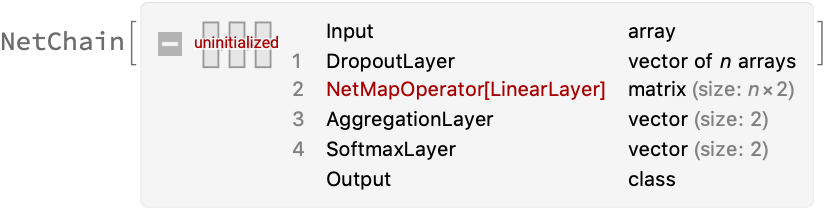
Define a network to classify the sequences of subword embeddings, using a max-pooling strategy:
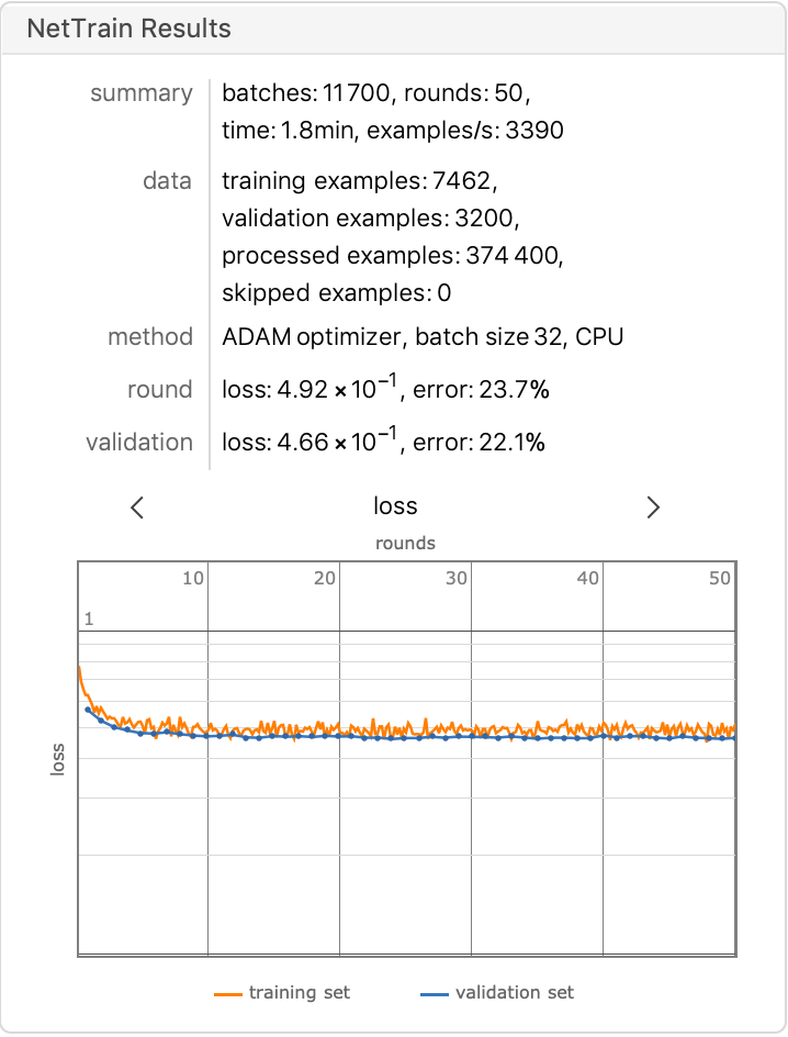
Train the network on the precomputed vectors from the pre-trained distilled BERT:
Check the classification error rate on the validation data:
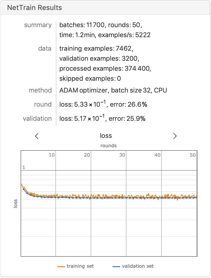
Compare the results with the performance of a classifier trained on context-independent word embeddings. Precompute the GloVe vectors for the training and the validation dataset:
Train the classifier on the precomputed GloVe vectors:
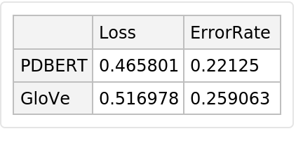
Compare the results obtained from the pre-trained distilled BERT with GloVe:
Net information
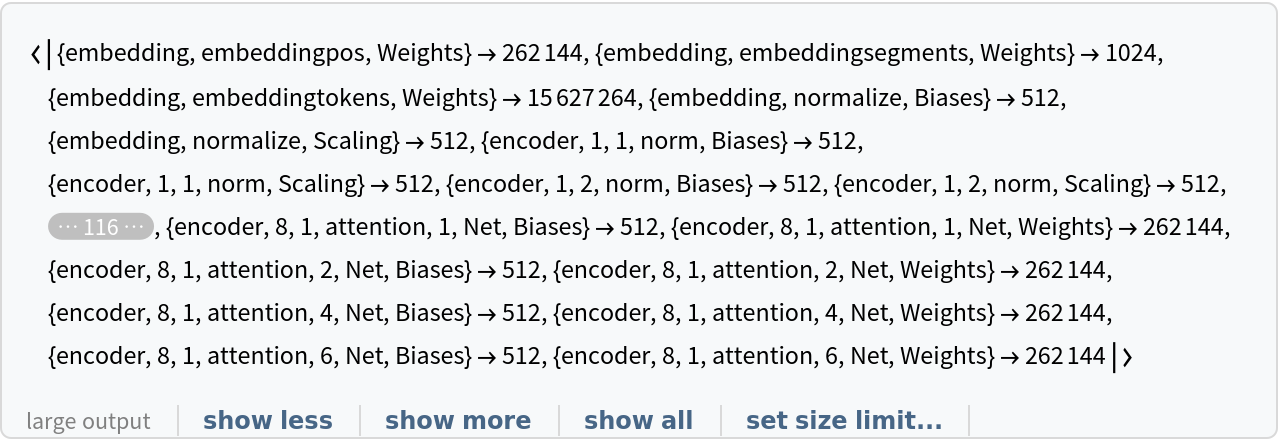
Inspect the number of parameters of all arrays in the net:
Obtain the total number of parameters:
Obtain the layer type counts:
Display the summary graphic:
Export to MXNet
Export the net into a format that can be opened in MXNet:
Export also creates a net.params file containing parameters:
Get the size of the parameter file:
![NetModel[{"Pre-trained Distilled BERT Trained on BookCorpus and \
English Wikipedia Data", "AttentionHeads" -> 4, "AttentionUnits" -> 12, "InputType" -> "ListOfStrings"}, "UninitializedEvaluationNet"]](https://www.wolframcloud.com/obj/resourcesystem/images/6f0/6f08647d-497c-4b10-9632-14cff52f0aaa/2963557f58b8fbcb.png)
![input = "Hello world! I am here";
embeddings = NetModel["Pre-trained Distilled BERT Trained on BookCorpus and \
English Wikipedia Data"][input];](https://www.wolframcloud.com/obj/resourcesystem/images/6f0/6f08647d-497c-4b10-9632-14cff52f0aaa/6ac7a5c8e1ea1e90.png)
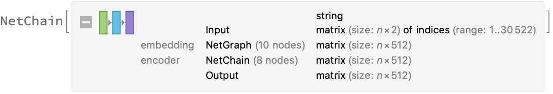
![net = NetModel[{"Pre-trained Distilled BERT Trained on BookCorpus and \
English Wikipedia Data", "InputType" -> "ListOfStrings"}];
netencoder = NetExtract[net, "Input"]](https://www.wolframcloud.com/obj/resourcesystem/images/6f0/6f08647d-497c-4b10-9632-14cff52f0aaa/24a020292c7001ba.png)
![embeddings = net[{"Hello world!", "I am here"},
{NetPort[{"embedding", "embeddingpos", "Output"}],
NetPort[{"embedding", "embeddingtokens", "Output"}],
NetPort[{"embedding", "embeddingsegments", "Output"}]}];
Map[MatrixPlot, embeddings]](https://www.wolframcloud.com/obj/resourcesystem/images/6f0/6f08647d-497c-4b10-9632-14cff52f0aaa/34c3745a49c025da.png)
![sentenceembedding = NetAppend[
NetModel["Pre-trained Distilled BERT Trained on BookCorpus and \
English Wikipedia Data"], "pooling" -> SequenceLastLayer[]]](https://www.wolframcloud.com/obj/resourcesystem/images/6f0/6f08647d-497c-4b10-9632-14cff52f0aaa/15a55505959c101b.png)


![trainembeddings = NetModel["Pre-trained Distilled BERT Trained on BookCorpus and \
English Wikipedia Data"][train[[All, 1]], TargetDevice -> "CPU"] -> train[[All, 2]];
validembeddings = NetModel["Pre-trained Distilled BERT Trained on BookCorpus and \
English Wikipedia Data"][valid[[All, 1]], TargetDevice -> "CPU"] -> valid[[All, 2]];](https://www.wolframcloud.com/obj/resourcesystem/images/6f0/6f08647d-497c-4b10-9632-14cff52f0aaa/1a2d9c963de1f223.png)
![classifierhead = NetChain[{DropoutLayer[], NetMapOperator[2], AggregationLayer[Max, 1], SoftmaxLayer[]}, "Output" -> NetDecoder[{"Class", {"negative", "positive"}}]]](https://www.wolframcloud.com/obj/resourcesystem/images/6f0/6f08647d-497c-4b10-9632-14cff52f0aaa/52dc42eb2645616b.png)
![pdbertresults = NetTrain[classifierhead, trainembeddings, All,
ValidationSet -> validembeddings,
TargetDevice -> "CPU",
MaxTrainingRounds -> 50]](https://www.wolframcloud.com/obj/resourcesystem/images/6f0/6f08647d-497c-4b10-9632-14cff52f0aaa/52548d60de4344e6.png)
![trainembeddingsglove = NetModel["GloVe 300-Dimensional Word Vectors Trained on Wikipedia \
and Gigaword 5 Data"][train[[All, 1]], TargetDevice -> "CPU"] -> train[[All, 2]];
validembeddingsglove = NetModel["GloVe 300-Dimensional Word Vectors Trained on Wikipedia \
and Gigaword 5 Data"][valid[[All, 1]], TargetDevice -> "CPU"] -> valid[[All, 2]];](https://www.wolframcloud.com/obj/resourcesystem/images/6f0/6f08647d-497c-4b10-9632-14cff52f0aaa/442e3d079ee5e86f.png)
![gloveresults = NetTrain[classifierhead, trainembeddingsglove, All,
ValidationSet -> validembeddingsglove,
TrainingStoppingCriterion -> <|"Criterion" -> "ErrorRate", "Patience" -> 50|>,
TargetDevice -> "CPU",
MaxTrainingRounds -> 50]](https://www.wolframcloud.com/obj/resourcesystem/images/6f0/6f08647d-497c-4b10-9632-14cff52f0aaa/720117299df5cb5d.png)
![Information[
NetModel["Pre-trained Distilled BERT Trained on BookCorpus and \
English Wikipedia Data"], "ArraysElementCounts"]](https://www.wolframcloud.com/obj/resourcesystem/images/6f0/6f08647d-497c-4b10-9632-14cff52f0aaa/0f53f1d94d42e7bc.png)
![Information[
NetModel["Pre-trained Distilled BERT Trained on BookCorpus and \
English Wikipedia Data"], "ArraysTotalElementCount"]](https://www.wolframcloud.com/obj/resourcesystem/images/6f0/6f08647d-497c-4b10-9632-14cff52f0aaa/4c05895269bc1ad2.png)
![Information[
NetModel["Pre-trained Distilled BERT Trained on BookCorpus and \
English Wikipedia Data"], "LayerTypeCounts"]](https://www.wolframcloud.com/obj/resourcesystem/images/6f0/6f08647d-497c-4b10-9632-14cff52f0aaa/79797520dde7be37.png)
![Information[
NetModel["Pre-trained Distilled BERT Trained on BookCorpus and \
English Wikipedia Data"], "SummaryGraphic"]](https://www.wolframcloud.com/obj/resourcesystem/images/6f0/6f08647d-497c-4b10-9632-14cff52f0aaa/2cd88e4a5ac2be90.png)
![jsonPath = Export[FileNameJoin[{$TemporaryDirectory, "net.json"}], NetModel["Pre-trained Distilled BERT Trained on BookCorpus and \
English Wikipedia Data"], "MXNet"]](https://www.wolframcloud.com/obj/resourcesystem/images/6f0/6f08647d-497c-4b10-9632-14cff52f0aaa/33b0070ec60325e2.png)