Multi-scale Context Aggregation Net
Trained on
PASCAL VOC2012 Data
Released in 2016, this is the first model featuring a systematic use of dilated convolutions for pixel-wise classification. A context aggregation module featuring convolutions with exponentially increasing dilations is appended to a VGG-style front end.
Number of layers: 53 |
Parameter count: 141,149,720 |
Trained size: 565 MB |
Examples
Resource retrieval
Get the pre-trained net:
Evaluation function
Write an evaluation function to handle padding and tiling of the input image:
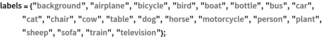
Label list
Define the label list for this model. Integers in the model’s output correspond to elements in the label list:
Basic usage
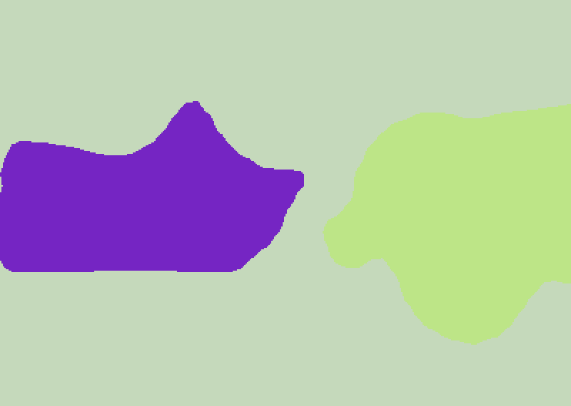
Obtain a segmentation mask for a given image:
Inspect which classes are detected:
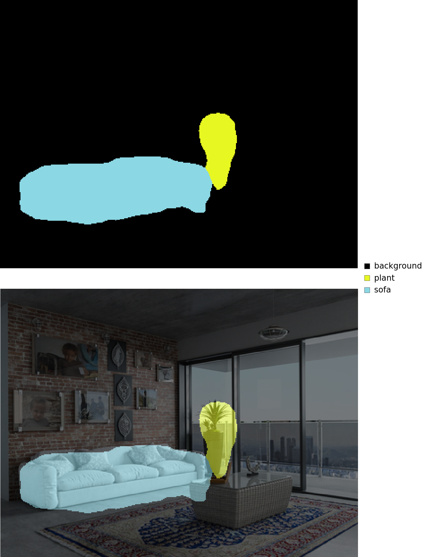
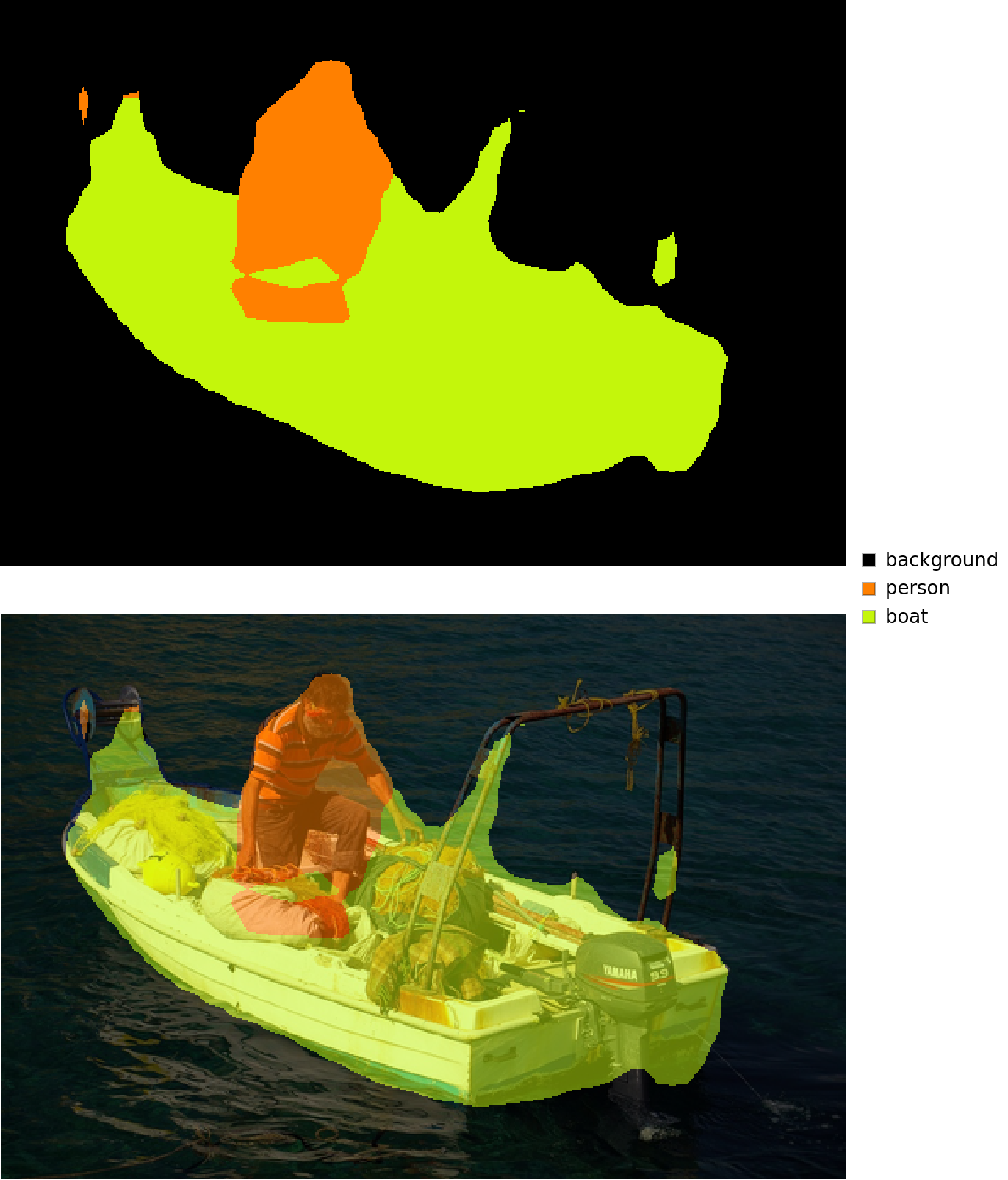
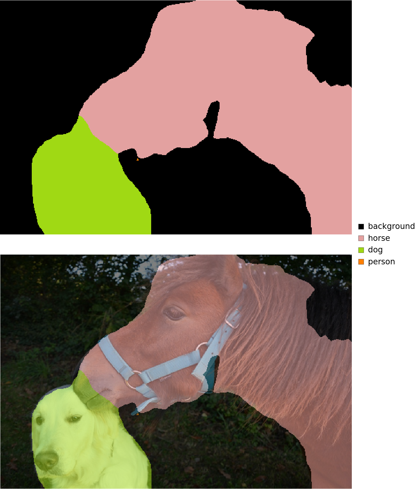
Visualize the mask:
Advanced visualization
Associate classes to colors:
Write a function to overlap the image and the mask with a legend:
Inspect the results:
Net information
Inspect the number of parameters of all arrays in the net:
Obtain the total number of parameters:
Obtain the layer type counts:
Export to MXNet
Export the net into a format that can be opened in MXNet:
Export also creates a net.params file containing parameters:
Get the size of the parameter file:
The size is similar to the byte count of the resource object:
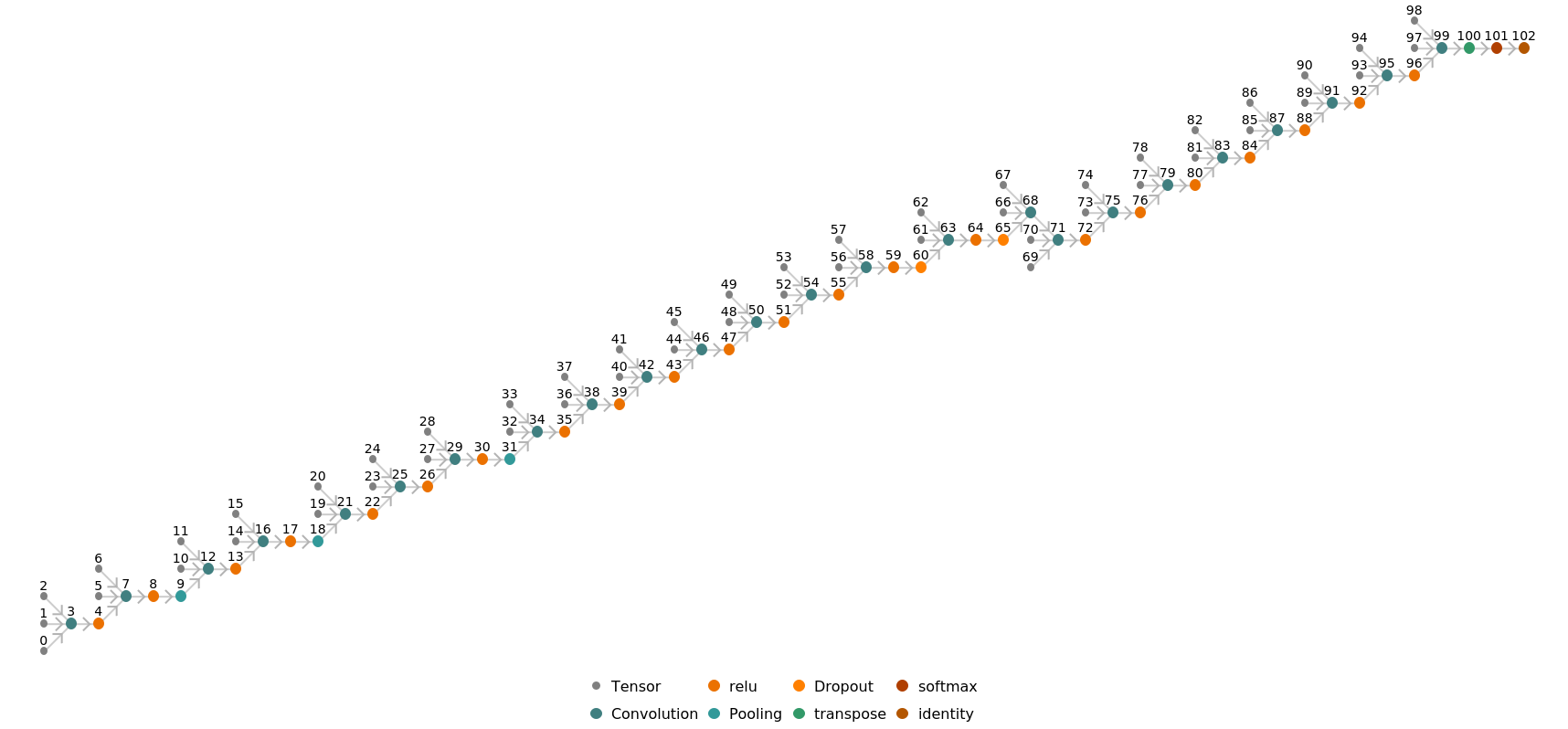
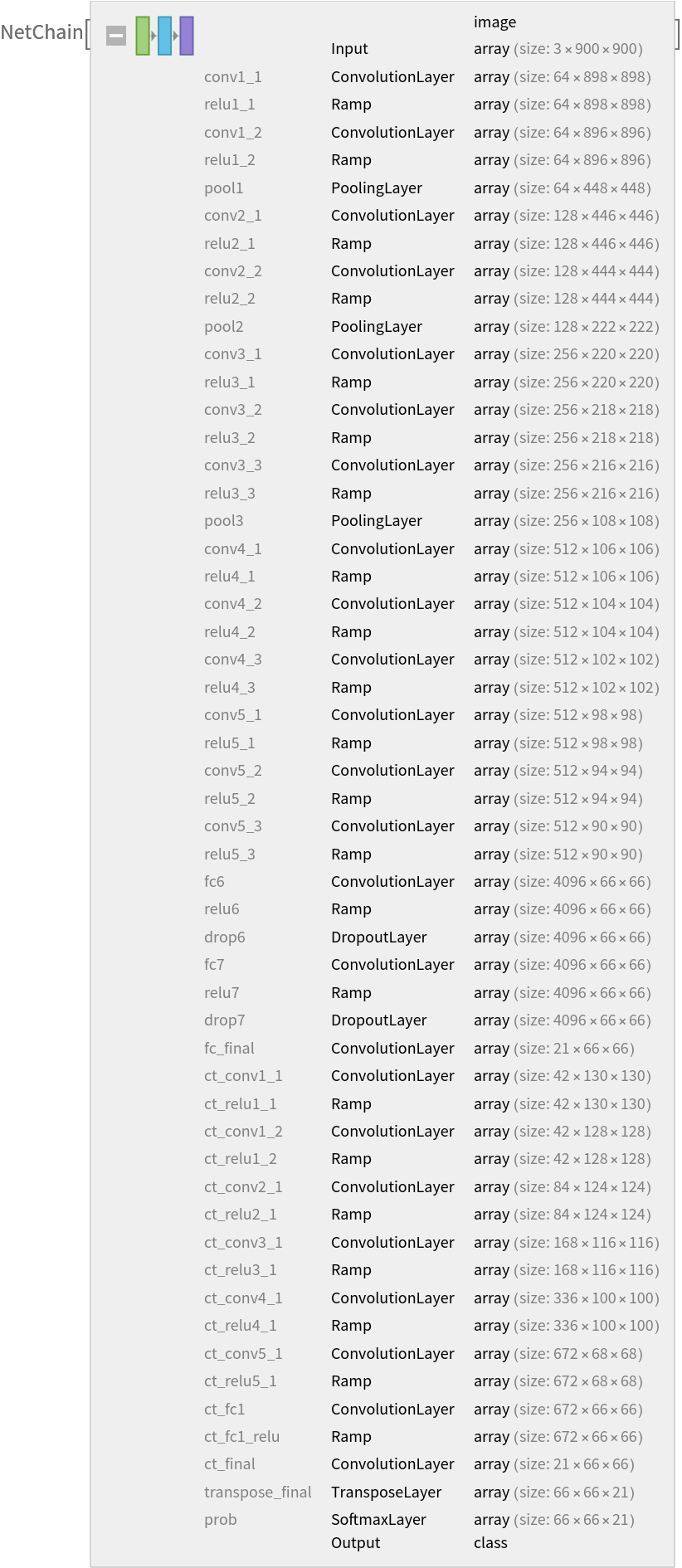
Represent the MXNet net as a graph:
Requirements
Wolfram Language
11.3
(March 2018)
or above
Resource History
Reference
![netevaluate[img_, device_ : "CPU"] := Block[
{net, marginImg, inputSize, windowSize, zoom, imgPad, imgSize, takeSpecs, tiles, marginTile, prob},
(* Parameters *)
net = NetModel[
"Multi-scale Context Aggregation Net Trained on PASCAL VOC2012 Data"];
marginImg = 186;
inputSize = 900;
zoom = 8;
windowSize = inputSize - 2*marginImg;
(* Pad and tile input *)
imgPad = ImagePad[img, marginImg, "Reflected"];
imgSize = ImageDimensions[imgPad];
takeSpecs = Table[
{{i, i + inputSize - 1}, {j, j + inputSize - 1}},
{i, 1, imgSize[[2]] - 2*marginImg, windowSize},
{j, 1, imgSize[[1]] - 2*marginImg, windowSize}
];
tiles = Map[ImageTake[imgPad, Sequence @@ #] &, takeSpecs, {2}];
(* Make all tiles 900x900 *)
marginTile = windowSize - Mod[imgSize - 2*marginImg, windowSize];
tiles = MapAt[ImagePad[#, {{0, marginTile[[1]]}, {0, 0}}, "Reflected"] &, tiles, {All, -1}];
tiles = MapAt[ImagePad[#, {{0, 0}, {marginTile[[2]], 0}}, "Reflected"] &, tiles, {-1, All}];
(* Run net on tiles *)
prob = net[Flatten@tiles, None, TargetDevice -> device];
prob = ArrayFlatten@
ArrayReshape[prob, Join[Dimensions@tiles, {66, 66, 21}]];
(* Resample probs by zoom factor and trim additional tile margin *)
prob = ArrayResample[prob, Dimensions[prob]*{zoom, zoom, 1}, Resampling -> "Linear"];
prob = Take[prob, Sequence @@ Reverse[ImageDimensions@img], All];
(* Predict classes *)
NetExtract[net, "Output"]@prob
]](https://www.wolframcloud.com/obj/resourcesystem/images/1ea/1ead5af1-b90a-45a0-be5e-857902d01daf/394d408a0ae1bf18.png)
![(* Evaluate this cell to get the example input *) CloudGet["https://www.wolframcloud.com/obj/3efa914d-9254-4e26-8d3e-b4cece2ecc05"]](https://www.wolframcloud.com/obj/resourcesystem/images/1ea/1ead5af1-b90a-45a0-be5e-857902d01daf/046dedfb70c93900.png)
![result[img_, device_ : "CPU"] := Block[
{mask, classes, maskPlot, composition},
mask = netevaluate[img, device];
classes = DeleteDuplicates[Flatten@mask];
maskPlot = Colorize[mask, ColorRules -> indexToColor];
composition = ImageCompose[img, {maskPlot, 0.5}];
Legended[
Row[Image[#, ImageSize -> Large] & /@ {maskPlot, composition}], SwatchLegend[indexToColor[[classes, 2]], labels[[classes]]]]
]](https://www.wolframcloud.com/obj/resourcesystem/images/1ea/1ead5af1-b90a-45a0-be5e-857902d01daf/3fd22933230bb0d9.png)
![(* Evaluate this cell to get the example input *) CloudGet["https://www.wolframcloud.com/obj/782161d3-f78f-4043-ae76-9fca90e5d651"]](https://www.wolframcloud.com/obj/resourcesystem/images/1ea/1ead5af1-b90a-45a0-be5e-857902d01daf/03d24b3e39238a8d.png)
![(* Evaluate this cell to get the example input *) CloudGet["https://www.wolframcloud.com/obj/2b4b42ea-eb73-4944-a3ad-8002af2843db"]](https://www.wolframcloud.com/obj/resourcesystem/images/1ea/1ead5af1-b90a-45a0-be5e-857902d01daf/335c07d550911682.png)
![(* Evaluate this cell to get the example input *) CloudGet["https://www.wolframcloud.com/obj/dc1d5cce-8c41-48e5-8e6c-4c6d5840829b"]](https://www.wolframcloud.com/obj/resourcesystem/images/1ea/1ead5af1-b90a-45a0-be5e-857902d01daf/2eba59b54ddf67f4.png)
![NetInformation[
NetModel[
"Multi-scale Context Aggregation Net Trained on PASCAL VOC2012 Data"], "ArraysElementCounts"]](https://www.wolframcloud.com/obj/resourcesystem/images/1ea/1ead5af1-b90a-45a0-be5e-857902d01daf/53f0a1557b5c099d.png)

![NetInformation[
NetModel[
"Multi-scale Context Aggregation Net Trained on PASCAL VOC2012 Data"], "ArraysTotalElementCount"]](https://www.wolframcloud.com/obj/resourcesystem/images/1ea/1ead5af1-b90a-45a0-be5e-857902d01daf/5efc17703ec80195.png)
![NetInformation[
NetModel[
"Multi-scale Context Aggregation Net Trained on PASCAL VOC2012 Data"], "LayerTypeCounts"]](https://www.wolframcloud.com/obj/resourcesystem/images/1ea/1ead5af1-b90a-45a0-be5e-857902d01daf/49e38314e15fcfb3.png)
![jsonPath = Export[FileNameJoin[{$TemporaryDirectory, "net.json"}], NetModel[
"Multi-scale Context Aggregation Net Trained on PASCAL VOC2012 Data"], "MXNet"]](https://www.wolframcloud.com/obj/resourcesystem/images/1ea/1ead5af1-b90a-45a0-be5e-857902d01daf/4b2a29df3d4770f4.png)