Multi-scale Context Aggregation Net
Trained on
CamVid Data
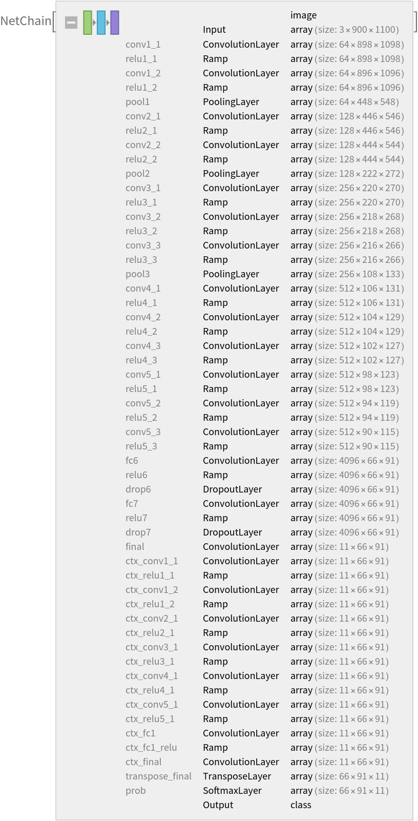
Released in 2016, this is the first model featuring a systematic use of dilated convolutions for pixel-wise classification. A context aggregation module featuring convolutions with exponentially increasing dilations is appended to a VGG-style front end.
Number of layers: 53 |
Parameter count: 134,313,443 |
Trained size: 537 MB |
Examples
Resource retrieval
Get the pre-trained net:
Evaluation function
Write an evaluation function to handle padding and tiling of the input image:
Label list
Define the label list for this model. Integers in the model’s output correspond to elements in the label list:
Basic usage
Obtain a segmentation mask for a given image:
Inspect which classes are detected:
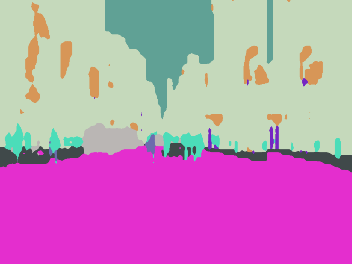
Visualize the mask:
Advanced visualization
Associate classes to colors:
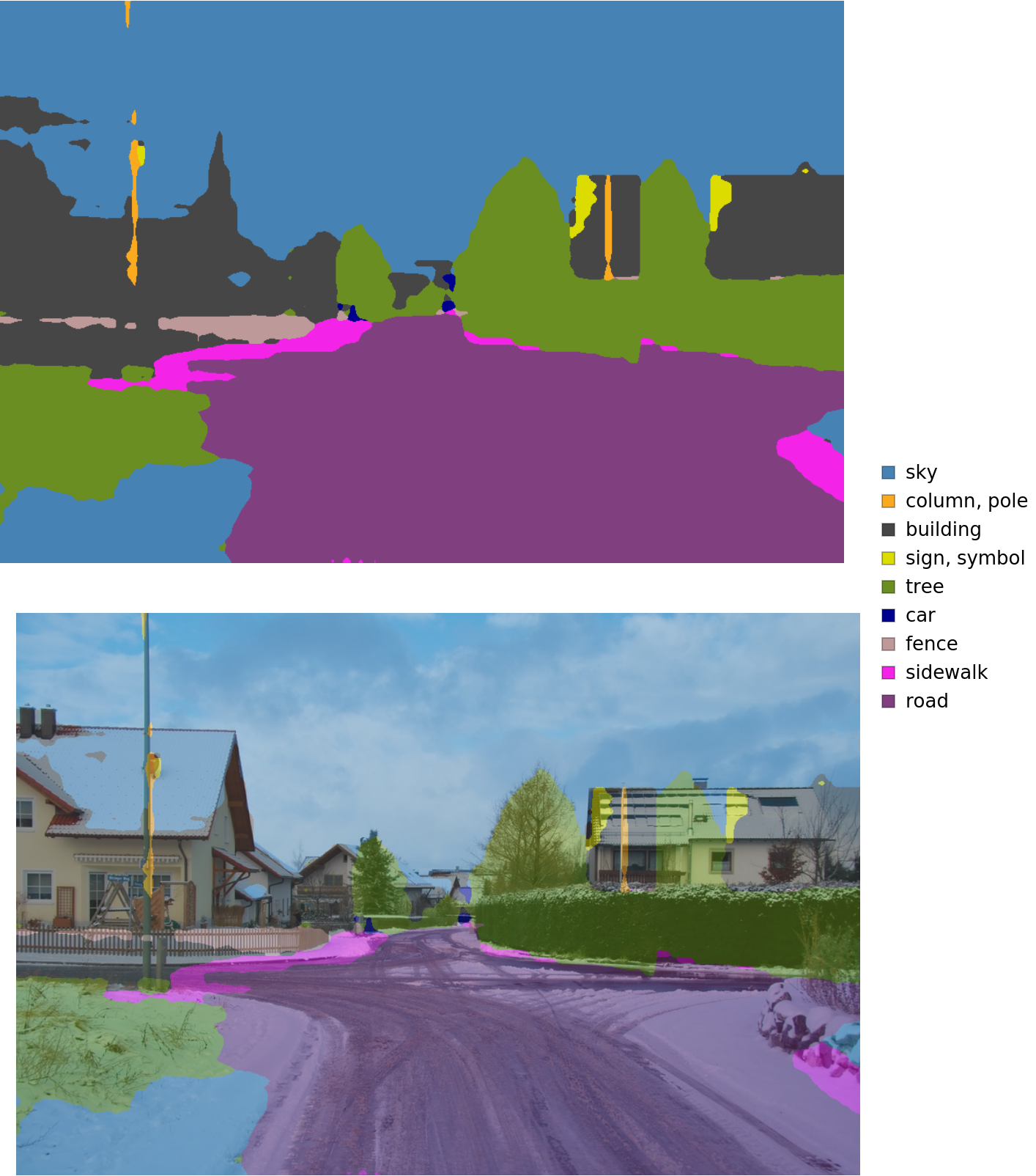
Write a function to overlap the image and the mask with a legend:
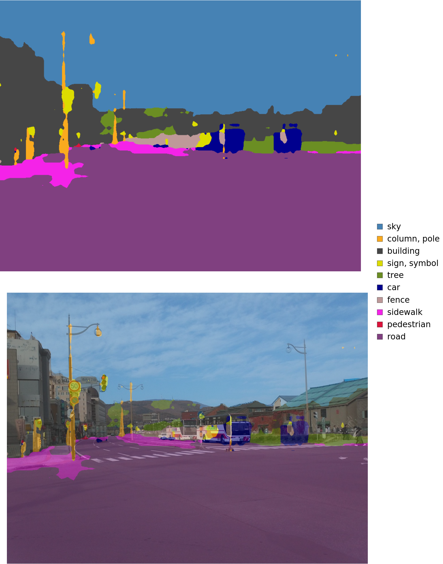
Inspect the results:
Net information
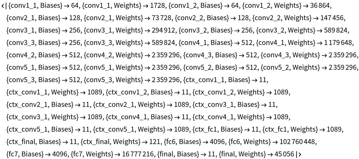
Inspect the number of parameters of all arrays in the net:
Obtain the total number of parameters:
Obtain the layer type counts:
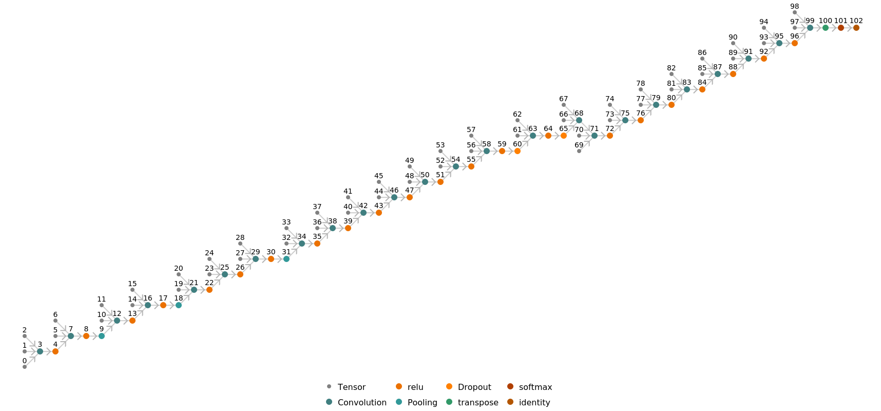
Display the summary graphic:
Export to MXNet
Export the net into a format that can be opened in MXNet:
Export also creates a net.params file containing parameters:
Get the size of the parameter file:
The size is similar to the byte count of the resource object:
Represent the MXNet net as a graph:
Requirements
Wolfram Language
11.3
(March 2018)
or above
Resource History
Reference
![netevaluate[img_, device_ : "CPU"] := Block[
{net, marginImg, inputSize, windowSize, zoom, imgPad, imgSize, takeSpecs, tiles, marginTile, prob},
(* Parameters *) net = NetModel[
"Multi-scale Context Aggregation Net Trained on CamVid Data"];
marginImg = 186;
inputSize = {900, 1100};
zoom = 8;
windowSize = inputSize - 2*marginImg;
(* Pad and tile input *) imgPad = ImagePad[img, marginImg, "Reflected"];
imgSize = ImageDimensions[imgPad];
takeSpecs = Table[
{{i, i + inputSize[[1]] - 1}, {j, j + inputSize[[2]] - 1}},
{i, 1, imgSize[[2]] - 2*marginImg, windowSize[[1]]},
{j, 1, imgSize[[1]] - 2*marginImg, windowSize[[1]]}
];
tiles = Map[ImageTake[imgPad, Sequence @@ #] &, takeSpecs, {2}];
(* Make all tiles 900x1100 *) marginTile = Reverse[windowSize] - Mod[imgSize - 2*marginImg, Reverse@windowSize];
tiles = MapAt[ImagePad[#, {{0, marginTile[[1]]}, {0, 0}}, "Reflected"] &, tiles, {All, -1}];
tiles = MapAt[ImagePad[#, {{0, 0}, {marginTile[[2]], 0}}, "Reflected"] &, tiles, {-1, All}];
(* Run net on tiles *) prob = net[Flatten@tiles, None, TargetDevice -> device];
prob = ArrayFlatten@
ArrayReshape[prob, Join[Dimensions@tiles, {66, 91, 11}]];
(* Resample probs by zoom factor and trim additional tile margin *) prob = ArrayResample[prob, Dimensions[prob]*{zoom, zoom, 1}, Resampling -> "Linear"];
prob = Take[prob, Sequence @@ Reverse[ImageDimensions@img], All];
(* Predict classes *)
NetExtract[net, "Output"]@prob
]](https://www.wolframcloud.com/obj/resourcesystem/images/8a7/8a711edb-ca16-4848-a16a-685dfe272ca9/164c15a322da01ec.png)
![(* Evaluate this cell to get the example input *) CloudGet["https://www.wolframcloud.com/obj/eba0964d-1078-4a01-b7b1-ea8b9afee76c"]](https://www.wolframcloud.com/obj/resourcesystem/images/8a7/8a711edb-ca16-4848-a16a-685dfe272ca9/455ddfb673caa781.png)
![colors = Apply[
RGBColor, {{70, 70, 70}, {107, 142, 35}, {70, 130, 180}, {0, 0, 142}, {220, 220, 0}, {128, 64, 128}, {220, 20, 60}, {190, 153, 153}, {250, 170, 30}, {244, 35, 232}, {119, 11, 32}}/255., {1}]](https://www.wolframcloud.com/obj/resourcesystem/images/8a7/8a711edb-ca16-4848-a16a-685dfe272ca9/34d3a4a67db730ac.png)
![result[img_, device_ : "CPU"] := Block[
{mask, classes, maskPlot, composition},
mask = netevaluate[img, device];
classes = DeleteDuplicates[Flatten@mask];
maskPlot = Colorize[mask, ColorRules -> indexToColor];
composition = ImageCompose[img, {maskPlot, 0.5}];
Legended[
Row[Image[#, ImageSize -> Large] & /@ {maskPlot, composition}], SwatchLegend[indexToColor[[classes, 2]], labels[[classes]]]]
]](https://www.wolframcloud.com/obj/resourcesystem/images/8a7/8a711edb-ca16-4848-a16a-685dfe272ca9/17eedda7bc57576d.png)
![(* Evaluate this cell to get the example input *) CloudGet["https://www.wolframcloud.com/obj/77c48e7d-651a-47dc-b45a-3955ef330620"]](https://www.wolframcloud.com/obj/resourcesystem/images/8a7/8a711edb-ca16-4848-a16a-685dfe272ca9/275c0a86559ed5c4.png)
![(* Evaluate this cell to get the example input *) CloudGet["https://www.wolframcloud.com/obj/ef029a30-5ea5-40b0-938a-0186d21dded0"]](https://www.wolframcloud.com/obj/resourcesystem/images/8a7/8a711edb-ca16-4848-a16a-685dfe272ca9/1406ce2122707c3a.png)