Resource retrieval
Get the pre-trained net:
NetModel parameters
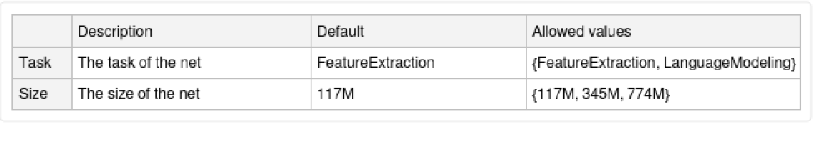
This model consists of a family of individual nets, each identified by a specific parameter combination. Inspect the available parameters:
Pick a non-default net by specifying the parameters:
Pick a non-default uninitialized net:
Basic usage
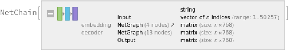
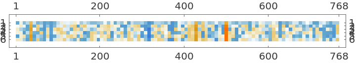
Given a piece of text, the GPT-2 net produces a sequence of feature vectors of size 768, which corresponds to the sequence of input words or subwords:
Obtain dimensions of the embeddings:
Visualize the embeddings:
Transformer architecture
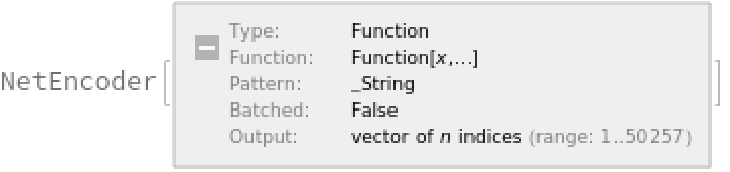
The input string is first normalized and then tokenized, or split into words or subwords. This two-step process is accomplished using the NetEncoder "Function":
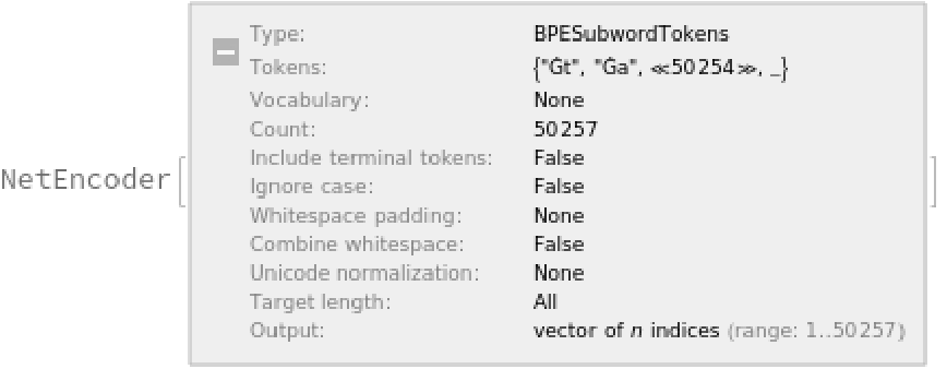
The tokenization step is performed using the NetEncoder "BPESubwordTokens" and can be extracted using the following steps:
The encoder produces an integer index for each subword token that corresponds to the position in the vocabulary:
Each subword token is also assigned a positional index:
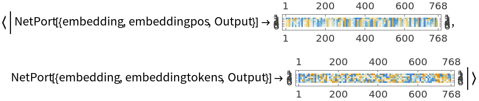
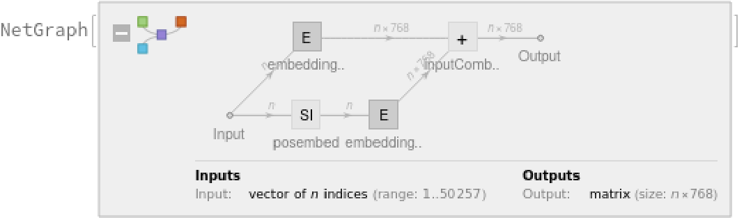
A lookup is done to map these indices to numeric vectors of size 768:
For each subword token, these two embeddings are combined by summing elements with ThreadingLayer:
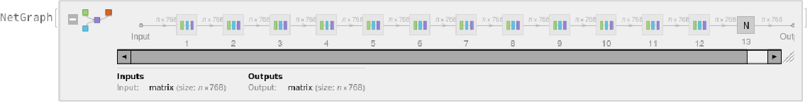
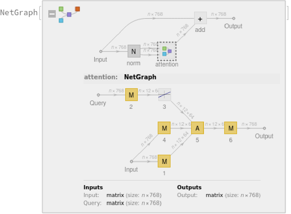
The transformer architecture then processes the vectors using 12 structurally identical self-attention blocks stacked in a chain:
The key part of these blocks is the attention module comprising of 12 parallel self-attention transformations, also called “attention heads”:
Attention is done with causal masking, which means that the embedding of a given subword token depends on the previous subword tokens and not on the next ones.
This is a prerequisite to be able to generate text with the language model. The following figures compare causal attention to other forms of connectivity between input tokens:
Language modeling
Retrieve the language model by specifying the "Task" parameter:
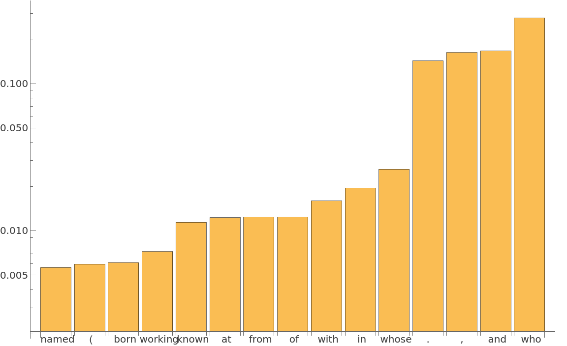
Predict the next word in a given sequence:
Obtain the top 15 probabilities:
Plot the top 15 probabilities:
Text generation
Define a function to predict the next token:
Generate the next 20 tokens by using it on a piece of text:
The third optional argument is a “temperature” parameter that scales the input to the final softmax. A high temperature flattens the distribution from which tokens are sampled, increasing the probability of extracting less likely tokens:
Decreasing the temperature sharpens the peaks of the sampling distribution, further decreasing the probability of extracting less likely tokens:
Very high temperature settings are equivalent to random sampling:
Very low temperature settings are equivalent to always picking the character with maximum probability. It is typical for sampling to “get stuck in a loop”:
Efficient text generation
The text generation example in the previous section wastes computational resources because every time a new token is produced, the language model reads the entire generated string from the beginning. This means that generating new tokens is more and more costly as text generation progresses. This can be avoided by using NetUnfold:
Write a function to efficiently generate text using the unfolded net:
Generate the next 20 tokens efficiently by using it on a piece of text:
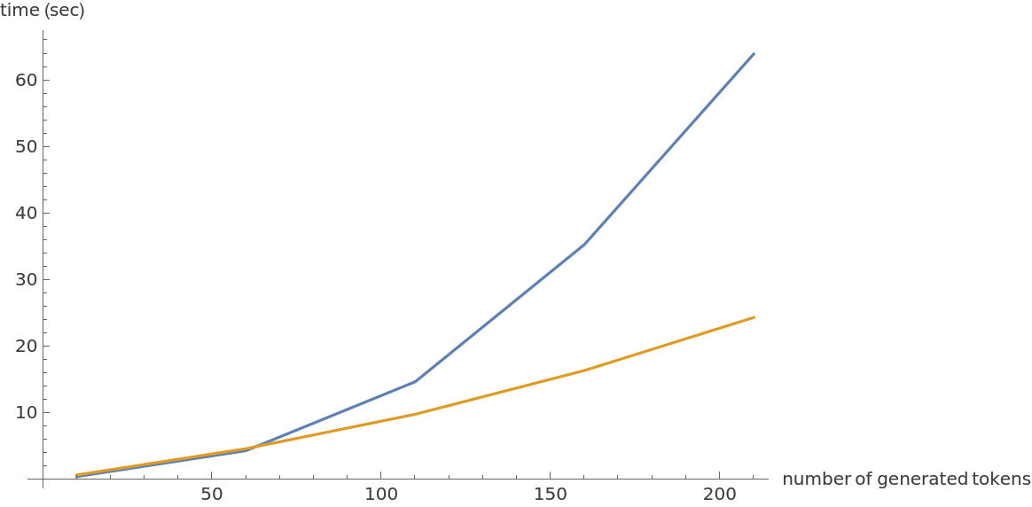
Compute the timings of the two methods for an increasing number of tokens:
Observe that the inefficient method grows quadratically with the number of tokens, while the efficient one is linear:
Sentence analogies
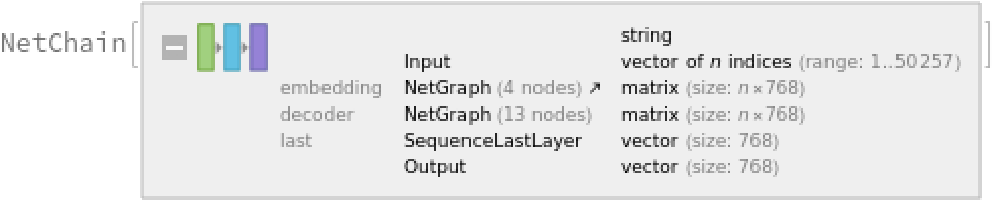
Define a sentence embedding that consists of the last subword embedding of GPT-2 (this choice is justified by the fact that GPT-2 is a forward causal model):
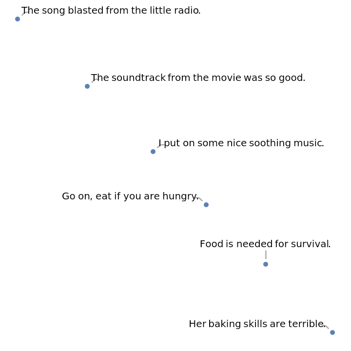
Define some sentences in two broad categories for comparison:
Precompute the embeddings for a list of sentences:
Visualize the similarity between the sentences using the net as a feature extractor:
Train a classifier model with the subword embeddings
Get a text-processing dataset:
View a random sample of the dataset:
Define a sentence embedding that consists of the last subword embedding of GPT-2 (this choice is justified by the fact that GPT-2 is a forward causal model):
Precompute the GPT-2 vectors for the training and the validation datasets (if available, GPU is recommended), using the last embedded vector as a representation of the entire text:
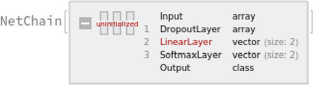
Define a simple network for classification:
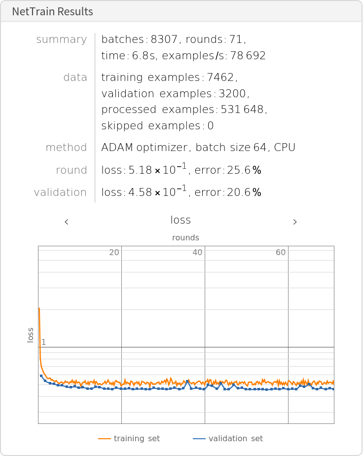
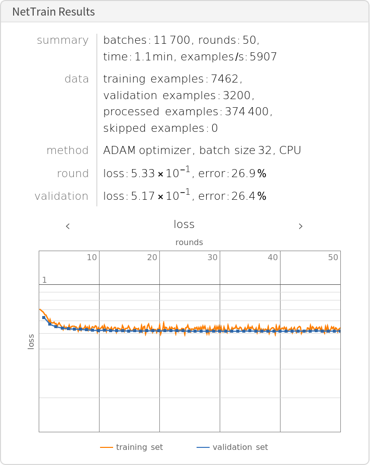
Train the network on the precomputed GPT-2 vectors:
Check the classification error rate on the validation data:
Compare the results with the performance of a classifier trained on context-independent word embeddings. Precompute the GloVe vectors for the training and the validation datasets (if available, GPU is recommended):
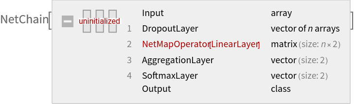
Define a simple network for classification using a max-pooling strategy:
Train the classifier on the precomputed GloVe vectors:
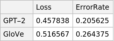
Compare the results obtained with GPT-2 and with GloVe:
Net information
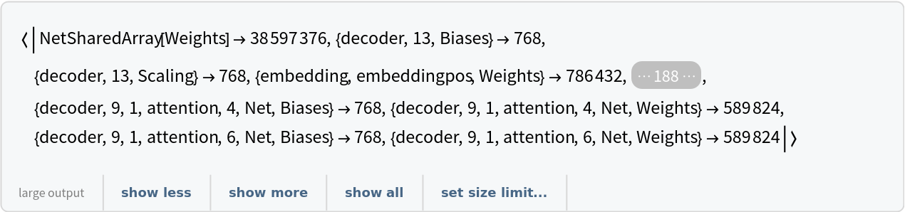
Inspect the number of parameters of all arrays in the net:
Obtain the total number of parameters:
Obtain the layer type counts:
Display the summary graphic:
Export to MXNet
Export the net into a format that can be opened in MXNet:
Export also creates a net.params file containing parameters:
Get the size of the parameter file:
![lm = NetModel[{"GPT2 Transformer Trained on WebText Data", "Task" -> "LanguageModeling", "Size" -> "345M"}]](https://www.wolframcloud.com/obj/resourcesystem/images/84d/84d61d0e-ae17-4af2-9e13-94be9545de84/759b65754eaf5057.png)
![NetModel[{"GPT2 Transformer Trained on WebText Data", "Task" -> "LanguageModeling"}, "UninitializedEvaluationNet"]](https://www.wolframcloud.com/obj/resourcesystem/images/84d/84d61d0e-ae17-4af2-9e13-94be9545de84/00e72619d72c9448.png)
![embeddings = net["Hello world! I am here",
{NetPort[{"embedding", "embeddingpos", "Output"}],
NetPort[{"embedding", "embeddingtokens", "Output"}]}];
Map[MatrixPlot, embeddings]](https://www.wolframcloud.com/obj/resourcesystem/images/84d/84d61d0e-ae17-4af2-9e13-94be9545de84/19c42b21f040a59e.png)
![topProbs = lm["Albert Einstein was a German-born theoretical physicist", {"TopProbabilities", 15}]](https://www.wolframcloud.com/obj/resourcesystem/images/84d/84d61d0e-ae17-4af2-9e13-94be9545de84/420ff97a99c26452.png)

![lm = NetModel[{"GPT2 Transformer Trained on WebText Data", "Task" -> "LanguageModeling"}];
generateSample[languagemodel_][input_String, numTokens_ : 10, temperature_ : 1] := Nest[Function[
StringJoin[#, languagemodel[#, {"RandomSample", "Temperature" -> temperature}]]],
input, numTokens];](https://www.wolframcloud.com/obj/resourcesystem/images/84d/84d61d0e-ae17-4af2-9e13-94be9545de84/64a3e44d5960fbce.png)


![lm = NetModel[{"GPT2 Transformer Trained on WebText Data", "Task" -> "LanguageModeling"}];
unfolded = NetUnfold[lm];
encoder = NetExtract[lm, "Input"];](https://www.wolframcloud.com/obj/resourcesystem/images/84d/84d61d0e-ae17-4af2-9e13-94be9545de84/32154ceff77f2e87.png)
![generateSampleEfficient[languagemodel_][input_String, numTokens_ : 10,
temperature_ : 1] := Block[
{encodedinput = encoder[input], index = 1, init, props, generated = {}},
init = Join[
<|"Input" -> First@encodedinput, "Index" -> index|>,
Association@Table["State" <> ToString[i] -> {}, {i, 24}]
];
props = Append[Table["OutState" <> ToString[i], {i, 24}], "Output" -> {"RandomSample", "Temperature" -> temperature}];
Nest[
Function@Block[
{newinput = KeyMap[StringReplace["OutState" -> "State"], languagemodel[#, props]]},
Join[newinput,
<|
"Index" -> ++index,
"Input" -> If[index <= Length[encodedinput],
encodedinput[[index]],
AppendTo[generated, newinput["Output"]];
Last@encoder@newinput["Output"]
]
|>
]
],
init,
numTokens + Length[encodedinput] - 1
];
StringJoin[input, generated]
];](https://www.wolframcloud.com/obj/resourcesystem/images/84d/84d61d0e-ae17-4af2-9e13-94be9545de84/35210714caaa4e8d.png)
![generateSampleEfficient[
unfolded]["Albert Einstein was a German-born theoretical physicist", 20]](https://www.wolframcloud.com/obj/resourcesystem/images/84d/84d61d0e-ae17-4af2-9e13-94be9545de84/0603b4e9e654be78.png)
![inefficientTimings = AssociationMap[
First@AbsoluteTiming[generateSample[lm]["I am", #]] &,
Range[10, 210, 50]
];
efficientTimings = AssociationMap[
First@
AbsoluteTiming[generateSampleEfficient[unfolded]["I am", #]] &,
Range[10, 210, 50]
];](https://www.wolframcloud.com/obj/resourcesystem/images/84d/84d61d0e-ae17-4af2-9e13-94be9545de84/553bc101ff3dd38a.png)
![ListLinePlot[{inefficientTimings, efficientTimings}, AxesLabel -> {"number of generated tokens", "time (sec)"}]](https://www.wolframcloud.com/obj/resourcesystem/images/84d/84d61d0e-ae17-4af2-9e13-94be9545de84/41b3a13985a9de24.png)
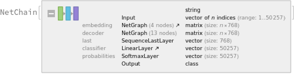
![sentenceembedding = NetAppend[NetModel["GPT2 Transformer Trained on WebText Data"], "last" -> SequenceLastLayer[]]](https://www.wolframcloud.com/obj/resourcesystem/images/84d/84d61d0e-ae17-4af2-9e13-94be9545de84/3e294804515e3aa9.png)

![train = ResourceData["Sample Data: Movie Review Sentence Polarity", "TrainingData"];
valid = ResourceData["Sample Data: Movie Review Sentence Polarity", "TestData"];](https://www.wolframcloud.com/obj/resourcesystem/images/84d/84d61d0e-ae17-4af2-9e13-94be9545de84/750163d3ed053c0f.png)
![sentenceembedding = NetAppend[NetModel["GPT2 Transformer Trained on WebText Data"], "last" -> SequenceLastLayer[]]](https://www.wolframcloud.com/obj/resourcesystem/images/84d/84d61d0e-ae17-4af2-9e13-94be9545de84/63116ef52c1e5f5f.png)
![classifierhead = NetChain[
{DropoutLayer[], 2, SoftmaxLayer[]},
"Output" -> NetDecoder[{"Class", {"negative", "positive"}}]
]](https://www.wolframcloud.com/obj/resourcesystem/images/84d/84d61d0e-ae17-4af2-9e13-94be9545de84/54172d1e461f7a39.png)
![gpt2results = NetTrain[classifierhead, trainembeddings, All,
ValidationSet -> validembeddings,
TrainingStoppingCriterion -> <|"Criterion" -> "ErrorRate", "Patience" -> 50|>,
TargetDevice -> "CPU",
MaxTrainingRounds -> 500]](https://www.wolframcloud.com/obj/resourcesystem/images/84d/84d61d0e-ae17-4af2-9e13-94be9545de84/72de83cfbb7c09bc.png)
![glove = NetModel[
"GloVe 300-Dimensional Word Vectors Trained on Wikipedia and Gigaword 5 Data"];](https://www.wolframcloud.com/obj/resourcesystem/images/84d/84d61d0e-ae17-4af2-9e13-94be9545de84/4dbeefa8a87dc8a0.png)
![gloveclassifierhead = NetChain[
{DropoutLayer[],
NetMapOperator[2],
AggregationLayer[Max, 1],
SoftmaxLayer[]},
"Output" -> NetDecoder[{"Class", {"negative", "positive"}}]]](https://www.wolframcloud.com/obj/resourcesystem/images/84d/84d61d0e-ae17-4af2-9e13-94be9545de84/103a9c398b2d59ec.png)
![gloveresults = NetTrain[gloveclassifierhead, trainembeddingsglove, All,
ValidationSet -> validembeddingsglove,
TrainingStoppingCriterion -> <|"Criterion" -> "ErrorRate", "Patience" -> 50|>,
TargetDevice -> "CPU",
MaxTrainingRounds -> 50]](https://www.wolframcloud.com/obj/resourcesystem/images/84d/84d61d0e-ae17-4af2-9e13-94be9545de84/1747524c82587640.png)
![Information[
NetModel[
"GPT2 Transformer Trained on WebText Data"], "ArraysElementCounts"]](https://www.wolframcloud.com/obj/resourcesystem/images/84d/84d61d0e-ae17-4af2-9e13-94be9545de84/50991b7fb5e2722d.png)
![Information[
NetModel[
"GPT2 Transformer Trained on WebText Data"], "ArraysTotalElementCount"]](https://www.wolframcloud.com/obj/resourcesystem/images/84d/84d61d0e-ae17-4af2-9e13-94be9545de84/727bb129ad315b05.png)
![jsonPath = Export[FileNameJoin[{$TemporaryDirectory, "net.json"}], NetModel["GPT2 Transformer Trained on WebText Data"], "MXNet"]](https://www.wolframcloud.com/obj/resourcesystem/images/84d/84d61d0e-ae17-4af2-9e13-94be9545de84/663e1bd433fb39e8.png)