Resource retrieval

Get the pre-trained net:

In[1]:=

Out[1]=

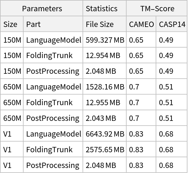
NetModel parameters

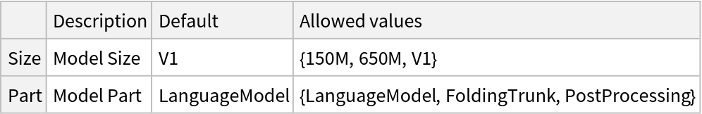
This model consists of a family of individual nets, each identified by a specific parameter combination. Inspect the available parameters:

In[2]:=

Out[2]=

Pick a non-default net by specifying the parameters:

In[3]:=

Out[3]=

Evaluation function

Write an evaluation function to scale the result to the input image size and suppress the least probable detections:

In[4]:=

In[5]:=

In[6]:=

In[7]:=

In[8]:=

Basic usage

Get a sequence:

In[9]:=

Obtain the sequence’s predicted structure:

In[10]:=

The detection includes the predicted structure and confidence score:

In[11]:=

Out[11]=

Plot the result:

In[12]:=

Out[12]=

Feature extraction

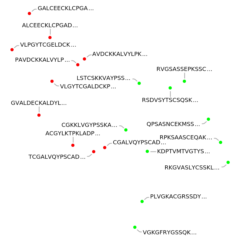
Define two sets of amino acid sequences originating from different protein families, namely enzymes and structural proteins:

In[13]:=

In[14]:=

Define the feature embeddings extractor using ESMFold:

In[15]:=

Visualize the features of the protein sequences:

In[16]:=

Out[16]=

Advanced usage

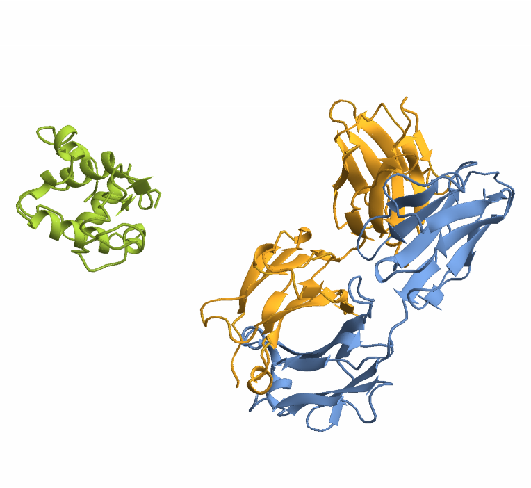
When working with proteins composed of multiple chains (multimers), a glycine linker (commonly 25 residues long) is automatically inserted between chains to create a single continuous sequence suitable for structure prediction. Glycine is typically chosen due to its small size and minimal structural impact. To demonstrate this, we’ll use the antibody 3HFM, which consists of three chains:

In[17]:=

Get the predicted structure and confidence score:

In[18]:=

In[19]:=

Out[19]=

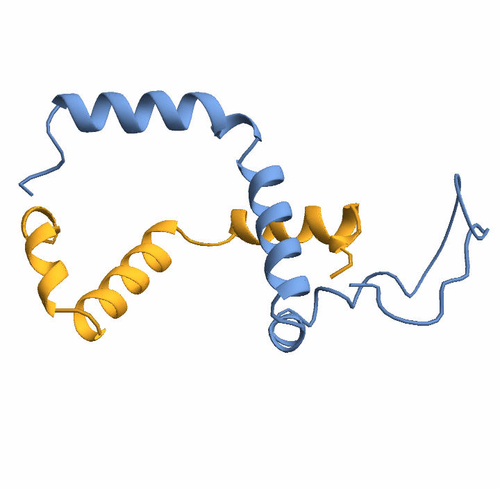
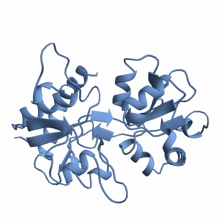
Visualize the structure:

In[20]:=

Out[20]=

Network result

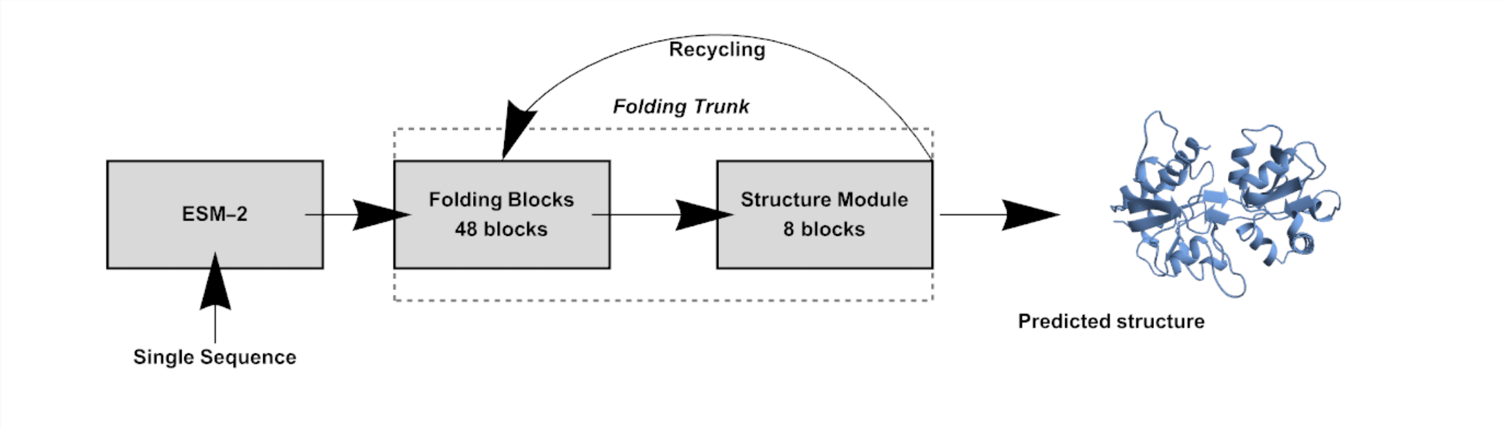
The following diagram shows the modular flow of the ESMFold inference process, which takes a protein sequence and outputs its 3D structure:

Out[50]=

The process starts with a raw amino acid sequence with two chains:

In[51]:=

The encodeSequence function converts the input protein sequence into numerical lists representing amino acid types, residue indices, a linker mask and chain identifiers for each residue:

In[52]:=

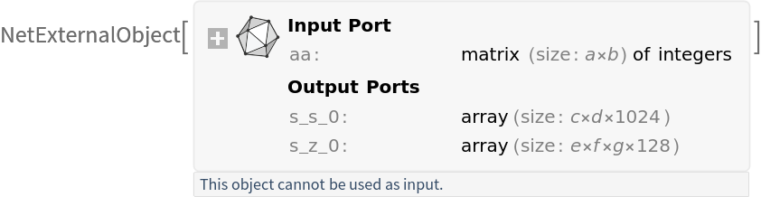
The pretrained ESM-2 language model extracts contextual embeddings from the input sequence:

In[53]:=

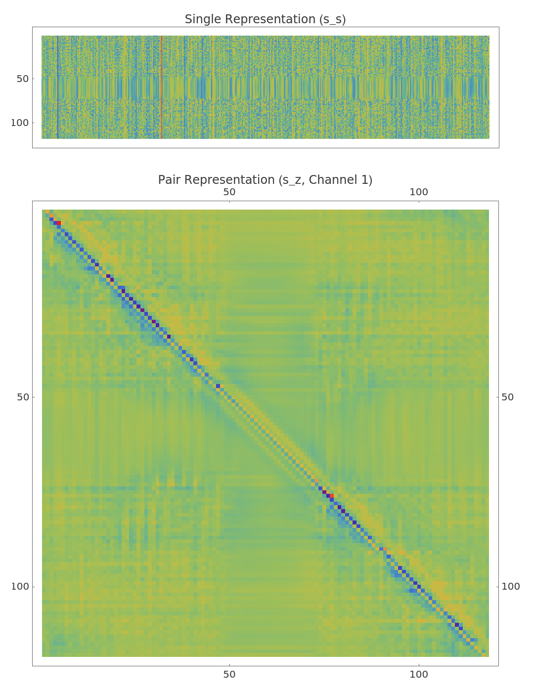
The result includes initial single (s_s_0) and pair (s_z_0) representations. The single representation encodes features for each residue, while the pair representation encodes features for every residue pair, enabling joint local and relational information during folding:

In[54]:=

Out[54]=

The Folding Trunk is a deep neural network composed of 48 Folding Blocks followed by an additional eight-block Structure Module; together, they refine the internal representations through multiple recycling steps, improving the predicted structure progressively. Initialize input metadata (mask and residue indices) and set up tensors for recycling intermediate representations:

In[55]:=

The recycling loop runs multiple times, each time passing the current representations and recycled values into the Folding Trunk model, which updates the representations and predicts the structure. Since the Folding Trunk model already includes the Structure Module internally, it returns both the refined internal features and the predicted atomic structure in a single call:

In[56]:=

Visualize the initial single and pair representations:

In[57]:=

Out[57]=

The post-processing part predicts the final atomic coordinates, frames, angles and sidechains. It also outputs the per-residue confidence (pLDDT) and prepares the data for visualization (PDB string):

In[58]:=

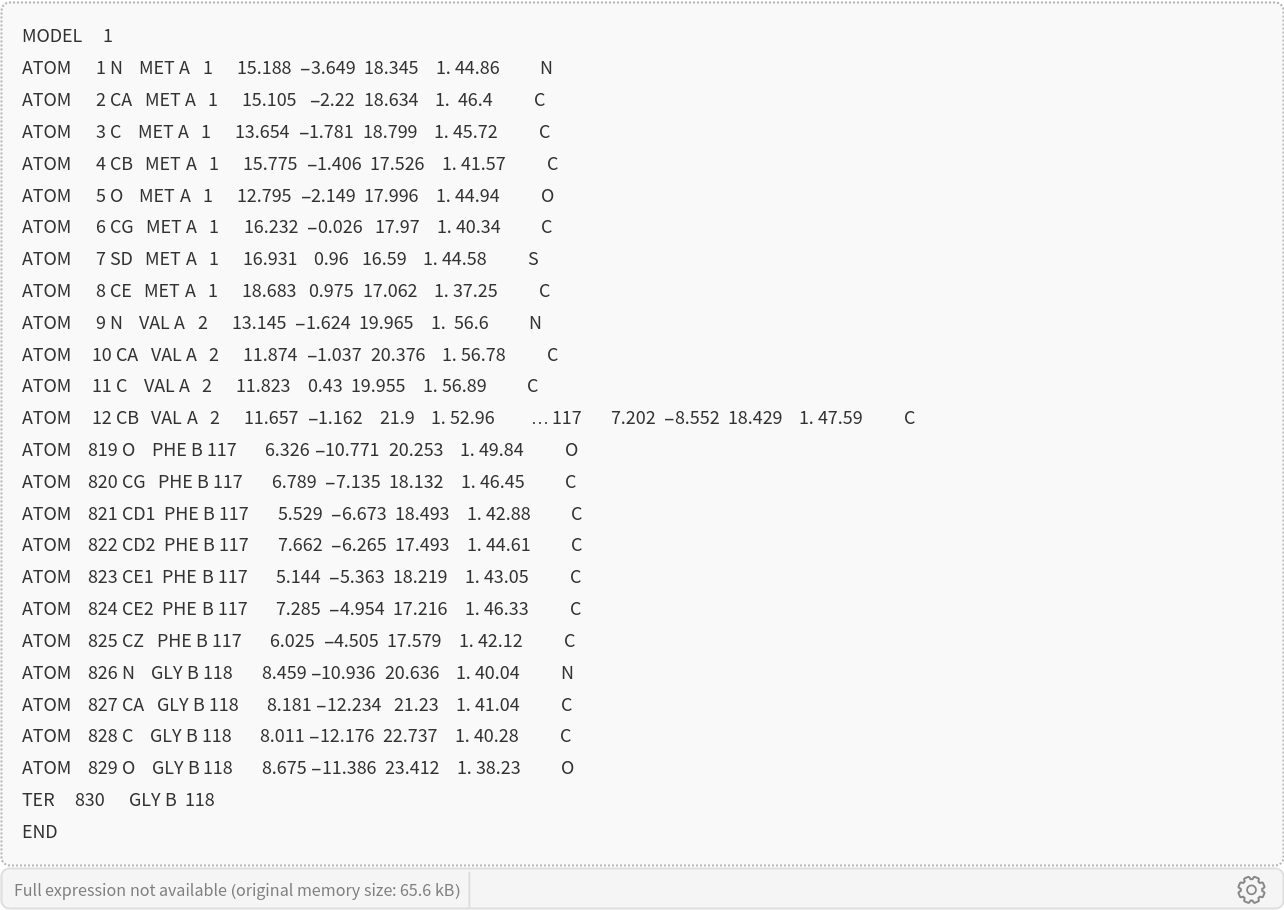
The final output includes atomic positions and confidence scores, used to render the 3D protein structure. Convert the output to PDB format:

In[59]:=

Out[59]=

Get the confidence score:

In[60]:=

Out[60]=

Plot the result:

In[61]:=

Out[61]=