Deep Speech 2
Trained on
Baidu English Data
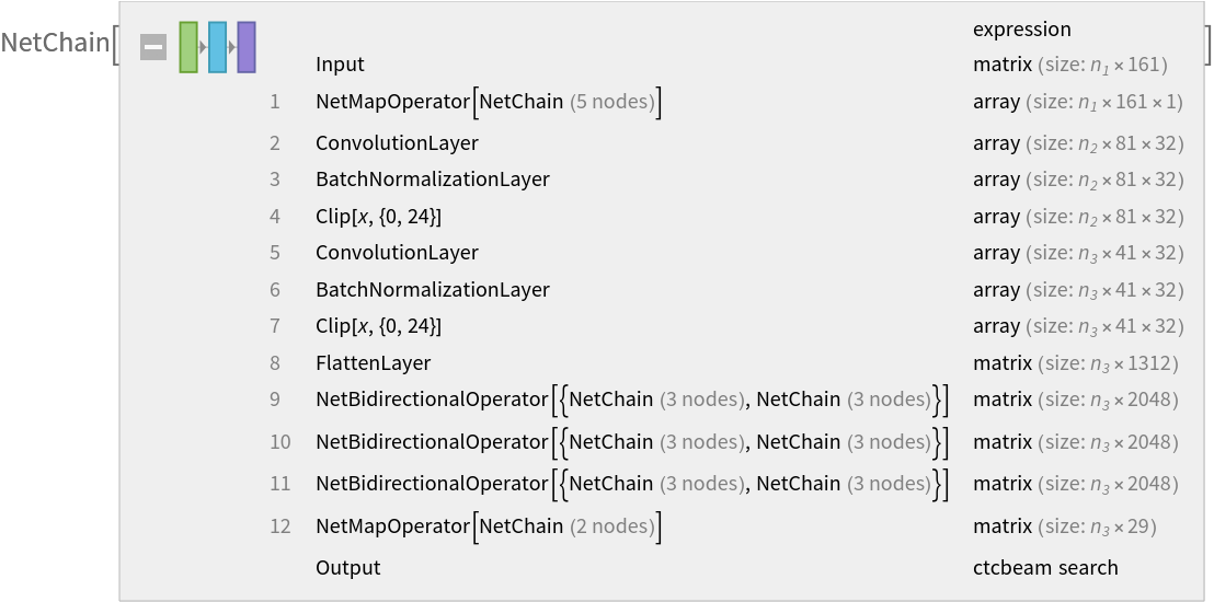
Released in 2015, Baidu Research's Deep Speech 2 model converts speech to text end to end from a normalized sound spectrogram to the sequence of characters. It consists of a few convolutional layers over both time and frequency, followed by gated recurrent unit (GRU) layers (modified with an additional batch normalization). At evaluation time, the space of possible output sequences is explored by the decoder using a beam search algorithm. The same architecture has also been shown to train successfully on Mandarin Chinese.
Number of layers: 152 |
Parameter count: 52,504,416 |
Trained size: 211 MB |
Examples
Resource retrieval
Get the pre-trained net:
Basic usage
Record an audio sample and transcribe it:
Join the characters:
Display the confidence of the five most likely hypotheses:
Performance evaluation
Models trained with CTC loss have difficulties in producing correct spelling:
The standard solution to this problem is to incorporate a language model into the beam search decoding procedure, as done in the original Deep Speech 2 implementation.
Noisy environments can affect the performance too:
Visualization
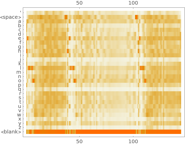
Write a function to visualize the token probabilities for each time step:
Inspect the character probabilities of the sample. The <blank> token is the standard blank token used by nets trained with CTC loss:
Net information
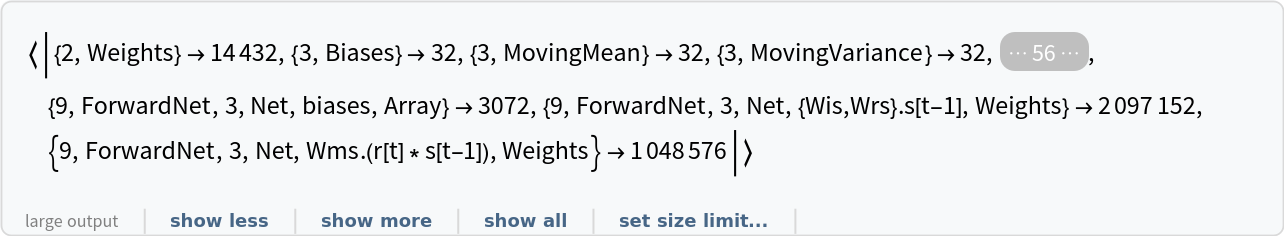
Inspect the sizes of all arrays in the net:
Obtain the total number of parameters:
Obtain the layer type counts:
Display the summary graphic:
Export to MXNet
Export the net into a format that can be opened in MXNet:
Export also creates a net.params file containing parameters:
Get the size of the parameter file:
The size is similar to the byte count of the resource object:
Requirements
Wolfram Language
11.3
(March 2018)
or above
Resource History
Reference
![(* Evaluate this cell to get the example input *) CloudGet["https://www.wolframcloud.com/obj/1e55f582-5a41-4684-94af-7230e63de91b"]](https://www.wolframcloud.com/obj/resourcesystem/images/90e/90e9550e-cae5-4879-b0f6-a5b32a71518f/121378a5e9a0fcf2.png)
![MapAt[StringJoin, NetModel["Deep Speech 2 Trained on Baidu English Data"][
record, {"TopNegativeLogLikelihoods", 5}], {All, 1}]](https://www.wolframcloud.com/obj/resourcesystem/images/90e/90e9550e-cae5-4879-b0f6-a5b32a71518f/70fc5a1f05fffbec.png)
![visualize[audio_] := With[{explikelihood = NetModel["Deep Speech 2 Trained on Baidu English Data"][audio, None]},
MatrixPlot[Transpose@explikelihood, FrameTicks -> {{Transpose@{Range[29], Join[{"'", "<space>"}, Alphabet[], {"<blank>"}]}, None}, {Automatic, Automatic}}, AspectRatio -> 0.8]
]](https://www.wolframcloud.com/obj/resourcesystem/images/90e/90e9550e-cae5-4879-b0f6-a5b32a71518f/3988b6b3c7710353.png)
![NetInformation[
NetModel[
"Deep Speech 2 Trained on Baidu English Data"], "ArraysTotalElementCount"]](https://www.wolframcloud.com/obj/resourcesystem/images/90e/90e9550e-cae5-4879-b0f6-a5b32a71518f/3bc9af45ea0072d5.png)

![jsonPath = Export[FileNameJoin[{$TemporaryDirectory, "net.json"}], NetModel["Deep Speech 2 Trained on Baidu English Data"], "MXNet"]](https://www.wolframcloud.com/obj/resourcesystem/images/90e/90e9550e-cae5-4879-b0f6-a5b32a71518f/2f18c339c677ef60.png)